If you missed our best recent articles:
250 Years of the US Economy - Part 1: Hamilton's Gamble (1776-1865)
The AI Token Economy, Tokenmaxxing & Physical AI Bottlenecks
“The risk of underinvesting is dramatically greater than the risk of overinvesting for us here.”
- Sundar Pichai, CEO of Alphabet, July 2024“For us, the risk of underinvesting is far greater than the risk of overinvesting.”
This statement explains the deepest driver of the AI cycle. For every hyperscaler, continuing to invest is a rational decision: spending too much may compress returns, but spending too little could cause the business to lose its technological edge for years to come. The problem arises when everyone reaches the same conclusion and simultaneously deploys unprecedented amounts of capital.
For most of the cycle, the equity market has focused on the question of how much growth AI can generate. The credit market is concerned with a different question: who will fund the build-out before that growth translates into cash?
The gap between these two questions is widening. Amazon, Alphabet, Microsoft, Meta, and Oracle entered the race with high profits, large cash piles, and some of the best access to capital in the world. However, hundreds of billions of dollars must still be spent on chips, data centers, networking, and power years before new capacity generates commensurate revenue.
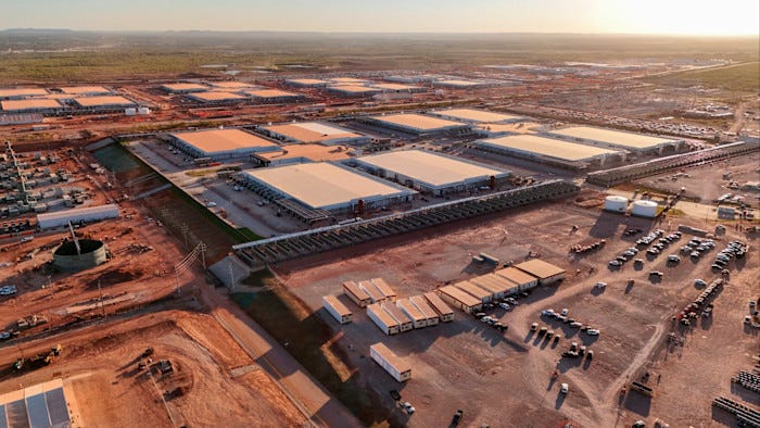
Therefore, the current risk is not yet a solvency crisis. It is primarily a problem of timing and capital absorption: capital expenditure is growing faster than operating cash flow, free cash flow is shrinking, and bonds, leases, and project financing are becoming the bridge between capital spent today and expected future revenue.
From the beginning of 2026 to the data cutoff date, the five hyperscalers issued approximately $194 billion in bonds, equivalent to nearly 9% of the investment-grade corporate bond supply within the tracked universe.
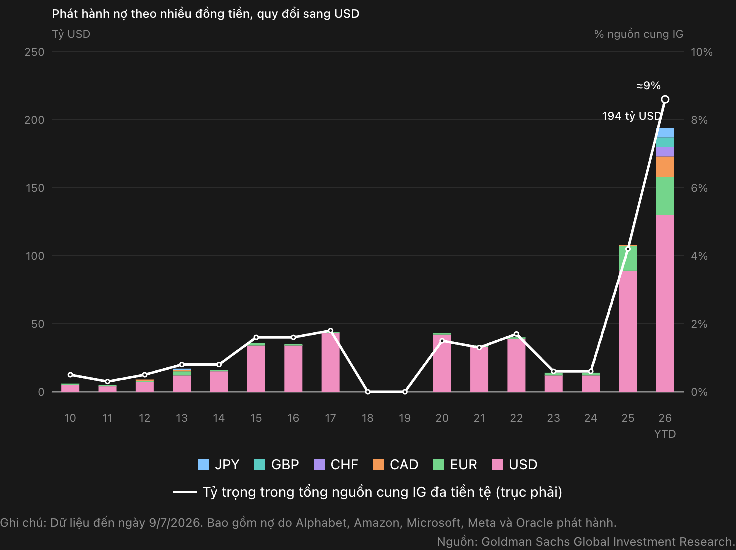
This scale raises three questions throughout this article:
Why do the world's most cash-rich companies need to borrow increasingly more?
Who will absorb the bond volume and interest rate risk arising from the AI race?
What happens if revenue eventually appears, but slower than the schedule of committed obligations?
AI credit is not yet a solvency crisis. It is primarily a capital absorption problem: a group of high-quality issuers is issuing increasingly large amounts of debt at longer maturities, while free cash flow is compressed by capex. Near-term risks are supply indigestion and funding selectivity. Macro risks only form if that pressure coincides with downward revisions to FCF, rising leverage, simultaneous tightening of multiple funding channels, and hyperscalers beginning to cut projects.
This is also where the interests of shareholders and creditors begin to diverge. Shareholders may accept years of investment if the final value is large enough. Bondholders do not share in that upside; their interests end at interest and principal payments, while the risks of additional issuance, credit rating deterioration, and widening yield spreads remain.
→ The article's thesis is not that AI is causing a debt crisis. The problem is that the pace of obligation accumulation has outstripped the pace of cash generation and is beginning to test the absorption limits of the financial system.
The first signal, therefore, may not be default, but an increasingly selective market: investors demanding higher compensation, better covenants, and more certain cash flows. The risk only turns into a broader shock if cash flow forecasts are simultaneously lowered, leverage continues to rise, and multiple funding channels tighten at once.
This week's Viethustler article will cover six parts:
Part I - Why capex has become a strategic commitment: investment scale, US-China competition, and why hyperscalers find it difficult to reduce spending.
Part II - The market must absorb duration, not just principal: AI issuance, DV01, cover ratio, spreads, and CDS.
Part III - The timing of free cash flow: consensus recovery, token economics, depreciation, and fixed commitments.
Part IV - When funding leaves the public bond market: leases, supplier debt, SPVs, project finance, and private credit.
Part V - KOSPI as an amplifier: when equity volatility becomes a macro signal.
Part VI - The three states of AI credit: supply indigestion, funding selectivity, and credit deterioration.
AI does not need to fail to be repriced.
Cash flow just needs to arrive slower than the pace at which the system accumulates obligations.
PART I - FROM TECH RACE TO CAPITAL DEMAND
1.1. Capex is absorbing the majority of operating cash flow
Previous computing cycles also required servers, networks, and data centers. But AI pushes capital intensity to another level: hardware is more expensive, power consumption is higher, and it requires an entire physical system to be built simultaneously.
An AI cluster needs more than just GPUs. It requires high-bandwidth memory, optical networking equipment, cooling systems, substations, land, power sources, and multi-year capacity contracts. Many items have lead times longer than the commercial lifecycle of the chips installed inside them.
The server memory market is an example. The spot price of DDR5 RDIMM32 rose 58.6% in 90 days to approximately $1,475 by mid-July 2026. The rally became evident from late May, just as demand for building AI infrastructure continued to expand.
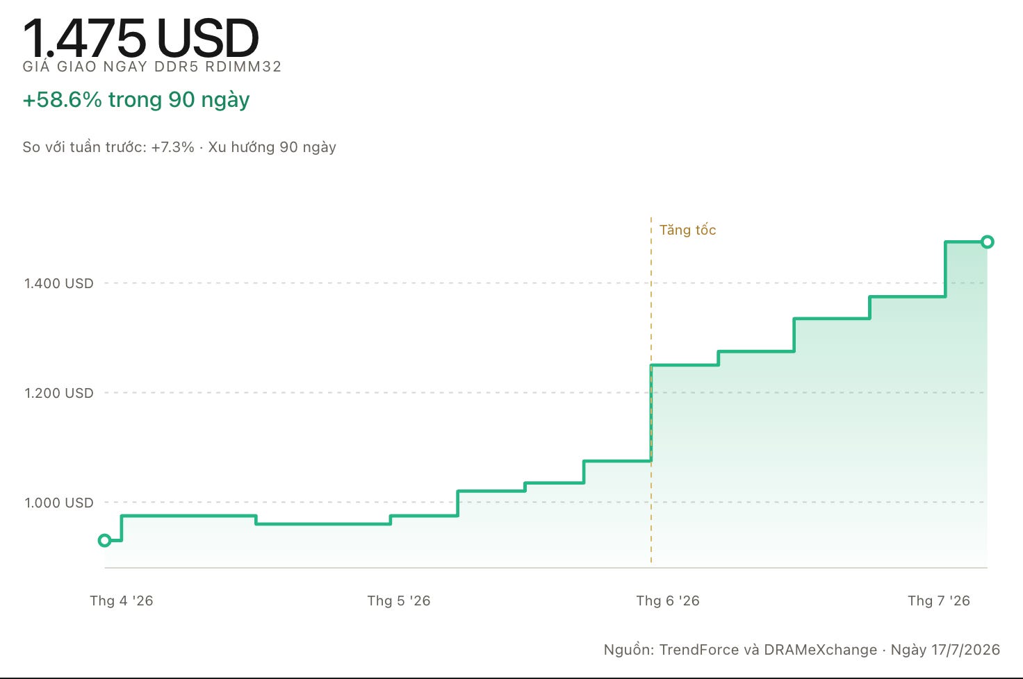
The chart does not represent the entire cost of a data center, but it shows an important characteristic of the current cycle: budgets can continue to rise even if capacity plans remain unchanged. When GPUs, memory, networking equipment, and power are all under pressure, the cost to complete a project will be higher than the initially approved figure.
This pressure manifests through three channels:
Rising component prices make the same amount of capacity more expensive.
Long deployment times force companies to pre-order and hold larger inventories.
Technological competition makes it difficult for hyperscalers to delay projects to wait for lower input prices.
That is why capital expenditure for the big tech group is rising along a rarely seen steep slope. The trailing 12-month capex of the Mag7 neared $450 billion at the end of the data series. Not all of this money is for AI, but the scale and growth rate show the race has shifted from software to physical infrastructure.
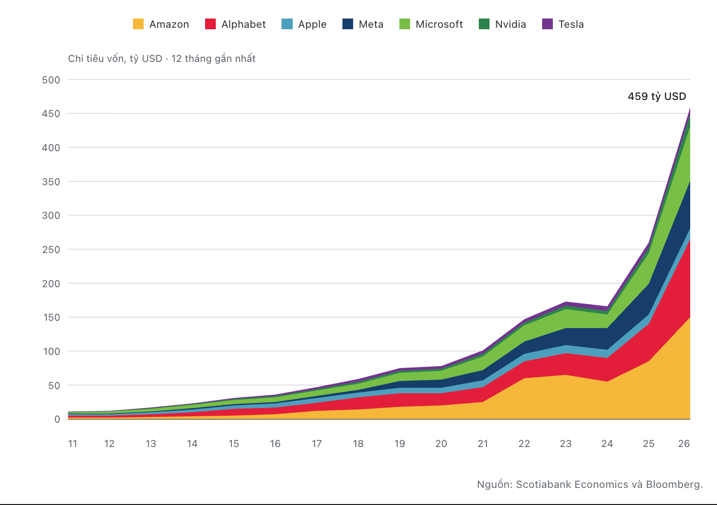
The important point lies in the sequence of cash flow. Companies must build capacity first, while revenue only appears after the data center goes live, customers deploy applications, and utilization levels are sufficiently high. This gap can be prolonged by:
long lead times for land, power, and networking equipment;
initial capacity often remaining underutilized;
new models potentially changing hardware configurations before old assets are amortized;
competition forcing companies to keep prices low to attract users and developers.
Pressure on cash flow has begun to show. Capex of AI hyperscalers was equivalent to only 49% of operating cash flow in 2024, but rose to 68% in 2025 and 75% in the 12 months ending in Q1 2026. According to consensus forecasts, this ratio could reach 94% for the full years 2026 and 2027.
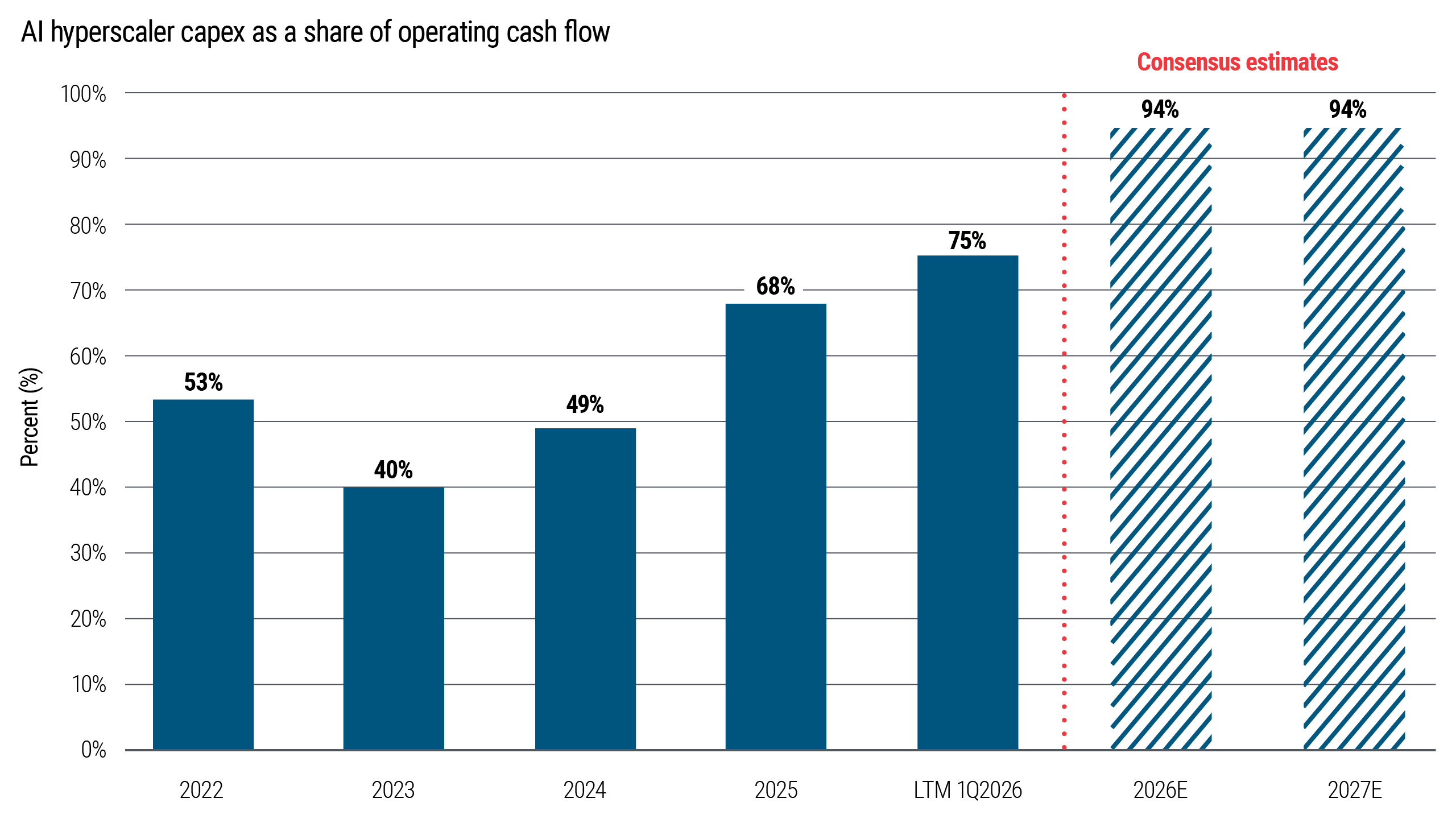
This does not mean hyperscalers are running out of cash. They still generate massive operating cash flow and have healthy balance sheets. But if nearly all of that cash must go back into infrastructure, the buffer for share buybacks, liquidity accumulation, and other projects will shrink significantly.
At that point, the ability to fund investment no longer depends solely on current profits. Bonds, leases, and project financing become the bridge between capital that must be spent today and revenue expected in the future.
→ The problem is not that capex is large, but that nearly all operating cash flow could be committed before the returns on new capacity are proven.
This is the first link that turns a tech story into a credit story.
1.2 The AI race makes capex a strategic commitment
In a normal investment cycle, companies can reduce spending when the cost of capital rises or demand weakens. In the AI race, that choice is much harder: saving capital today could mean losing a technological position for years to come.
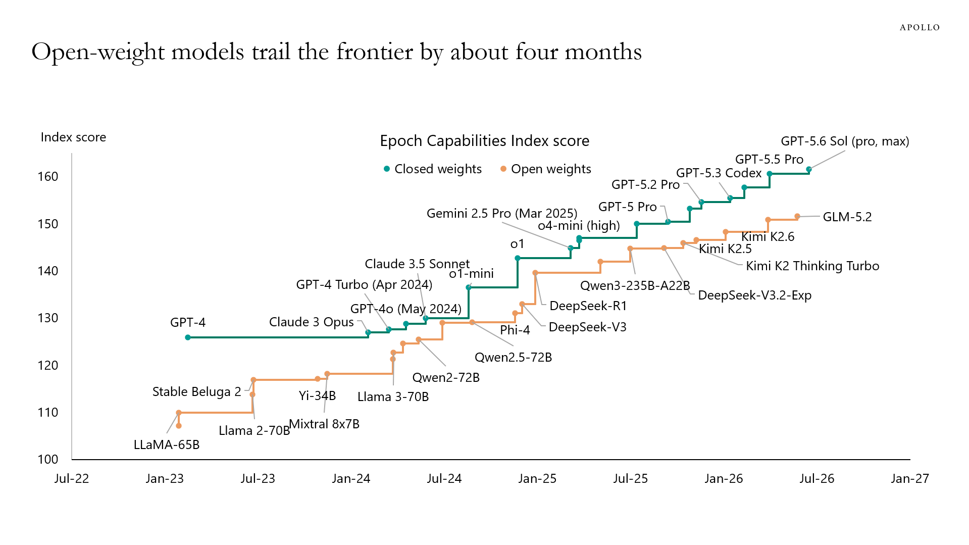
The capability gap between leading US and Chinese models has narrowed significantly since 2023. US models still lead, but the improvement pace of DeepSeek, Qwen, and Moonshot shows that the current advantage is not guaranteed if investment slows down.
Competitive pressure has also moved from the lab to usage levels. Among the top 20 AI models, the token volume of Chinese models increased from 46 trillion in May 2026 to 98 trillion in June, higher than the increase from 37 to 53 trillion for US models.
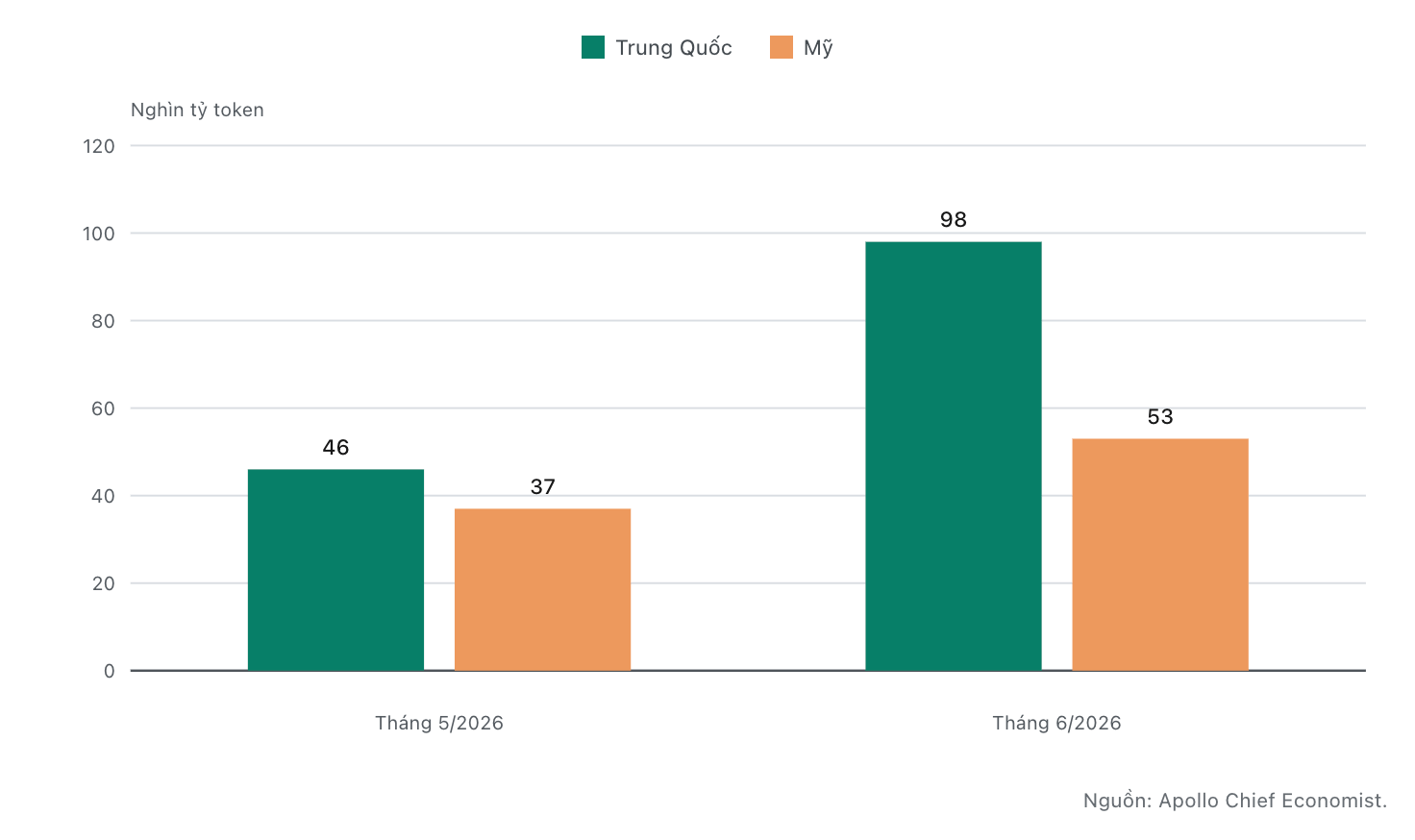
Two months of data are not enough to establish a long-term trend. Token volume does not equate to revenue, user numbers, or profit; it can increase due to low prices, open-source availability, API integration, or high inference volume with limited monetization potential.
Nevertheless, the competitive mechanism is clearer. US hyperscalers are not just protecting model quality, but must also protect:
the cloud ecosystem and their position in the distribution chain;
the stickiness of developers and enterprises;
cost advantages per unit of compute;
the right to shape future technology standards.
This makes capex inelastic. Even if short-term returns are unproven, the cost of stopping can be seen as greater than the cost of continuing to invest. At the same time, the popularity of low-priced models puts pressure on pricing power, risking that hardware savings are passed to customers instead of becoming supplier margins.
→ The AI race both reduces the ability to cut capex and raises the level of revenue that new capacity must generate to justify the capital already spent.
That is why the gap between investment and cash flow may persist longer than a typical construction cycle.
1.3 Balance sheets are still healthy, but the trajectory has changed
A deteriorating credit metric does not mean the balance sheet has become weak. For hyperscalers, it is important to separate direction of change from starting point.
This group entered the AI cycle with gross leverage of approximately 1.8x, net leverage of about 1.0x, a cash-to-debt ratio of 76%, and a median credit rating of AA-. Relatively long debt maturities also help mitigate short-term refinancing pressure.
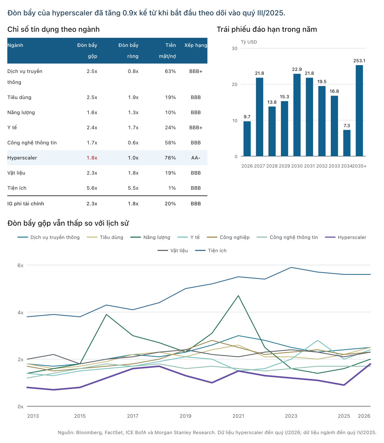
The gap with the rest of the market remains significant. Hyperscalers rated A or higher had historically maintained a net cash position and are not expected to shift to slightly positive net leverage until 2026. Even when considering the entire group, net leverage remains at only about 1.0x, compared to over 2.0x for the U.S. investment-grade (IG) corporate index.
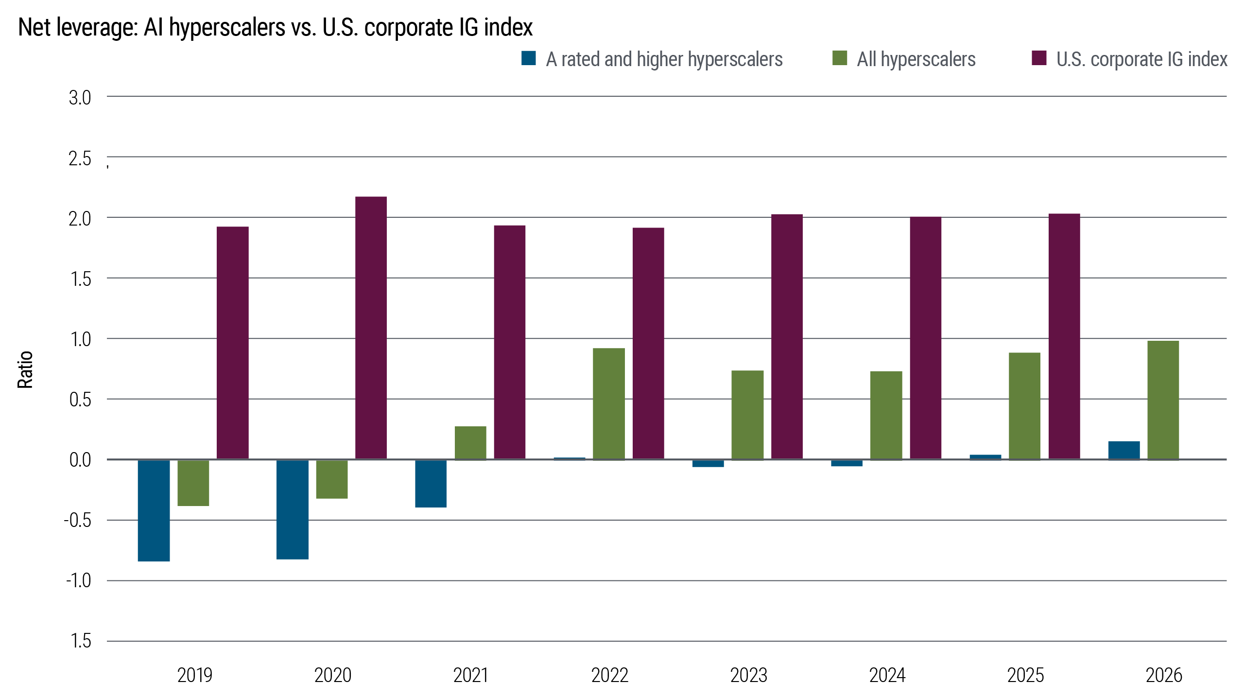
This foundation creates three layers of protection:
Highly rated issuers still have the capacity to borrow more without approaching the average IG leverage level.
Substantial cash reserves allow companies to endure a period of compressed free cash flow (FCF) without needing to cut capital expenditure (capex) immediately.
Management teams have numerous credit-protection tools at their disposal, ranging from reducing share buybacks to utilizing a mix of debt, equity, and project financing.
This is why the market has not faced a liquidity crisis. Hyperscalers are not borrowing to offset a failing business; they are using their strong balance sheets to deploy capital before new capacity generates revenue.
Theoretical financing capacity remains vast. Consensus forecasts place 2027 capex at approximately $920 billion, up 22% from 2026. In more aggressive scenarios, total cash flow from operations (CFO) and the absorption capacity of the IG market could support a scale of up to approximately $1.43 trillion.
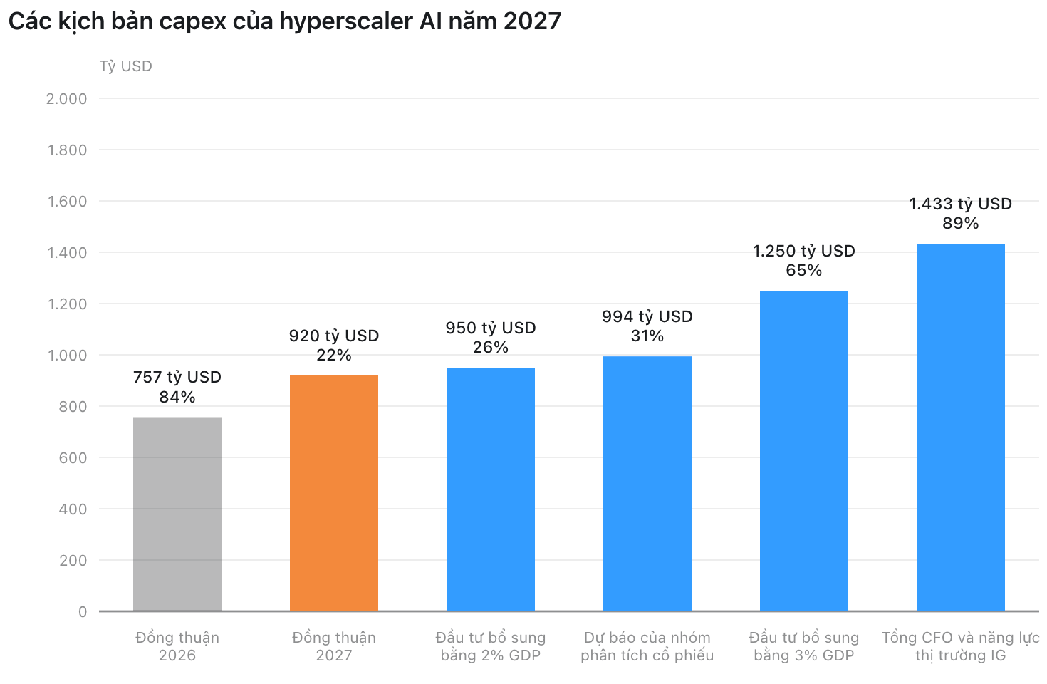
The $1.43 trillion figure is not a capex forecast, nor does it guarantee the market will provide that entire amount of capital at current costs. It is a scenario regarding financing capacity, suggesting the AI cycle could continue for longer before balance sheets become a hard constraint.
However, the ability to borrow more does not mean companies should borrow at any price. As long as FCF has not recovered, each new issuance increases interest expenses, fixed obligations, and market dependency. Investors will therefore gradually shift their focus to:
the ability to cover interest and fixed obligations;
leverage after adjusting for lease obligations;
the rate of debt growth relative to CFO and FCF;
the flexibility to reduce share buybacks or defer projects.
→ The positive takeaway is that hyperscalers have enough capacity to fund the AI race for several years; the point to monitor is that each year of pre-cash-flow investment erodes that buffer.
Therefore, the accurate thesis is not that Big Tech is nearing a debt crisis. The critical shift is that companies that were once nearly independent of the credit market are becoming frequent issuers.
The balance sheet determines how much they can borrow. In the next part of this article, we will examine at what price the market is willing to absorb that capital.
PART II - THE MARKET MUST ABSORB DURATION, NOT JUST PRINCIPAL
2.1. AI supply is accounting for an increasingly large share
A large issuance rarely destabilizes the market. Risk emerges when the same group of companies returns repeatedly, extending maturities and competing with a large volume of bonds from the rest of the economy.
AI-related debt supply has increased from approximately $25 billion in 2024 to nearly $240 billion year-to-date in 2026, equivalent to about 18% of the investment-grade bond supply within the tracked corporate universe.
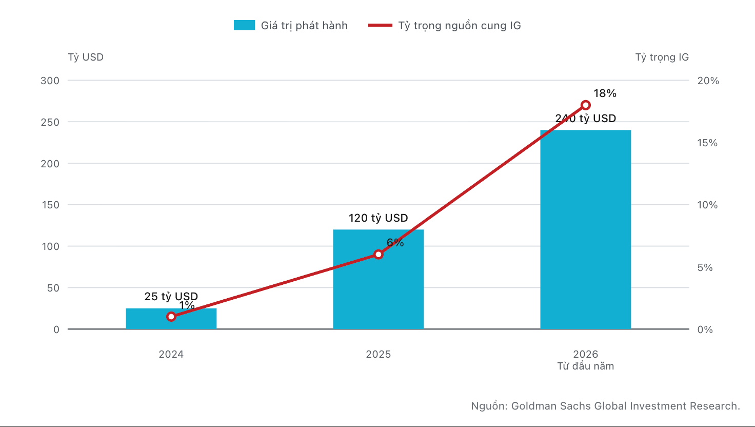
The $240 billion figure does not contradict the $194 billion mentioned in the introduction. The former uses a broader group, including semiconductor and related infrastructure companies; the latter counts only the five hyperscalers and aggregates issuances across multiple currencies. The two datasets answer different questions and are not interchangeable.
Pressure is also heavily concentrated at the long end of the curve. AI-related debt now accounts for over 40% of IG bonds with maturities of 15 years or longer, compared to about 5% in 2024.
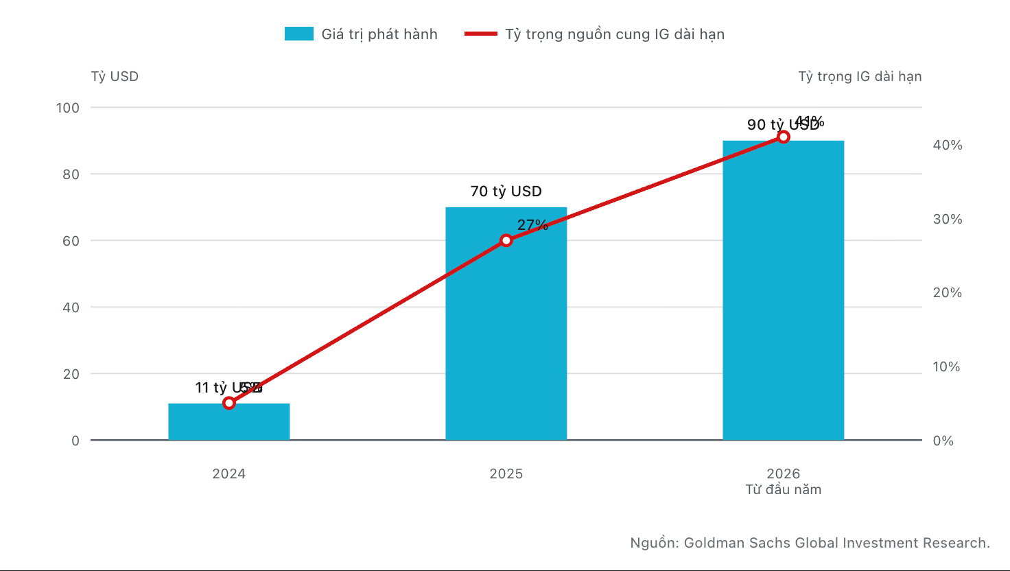
This concentration creates a risk trade-off. Companies reduce their short-term refinancing needs, but bond funds, insurance companies, and pension funds must hold additional interest rate risk for decades. Absorption capacity may therefore hit allocation limits before any company faces payment difficulties.
The broader environment is also less favorable. Total net issuance of fixed-income products in the U.S. is projected to rise from approximately $1.7 trillion in 2025 to over $2.3 trillion in 2026, with IG supply alone potentially approaching $1 trillion.
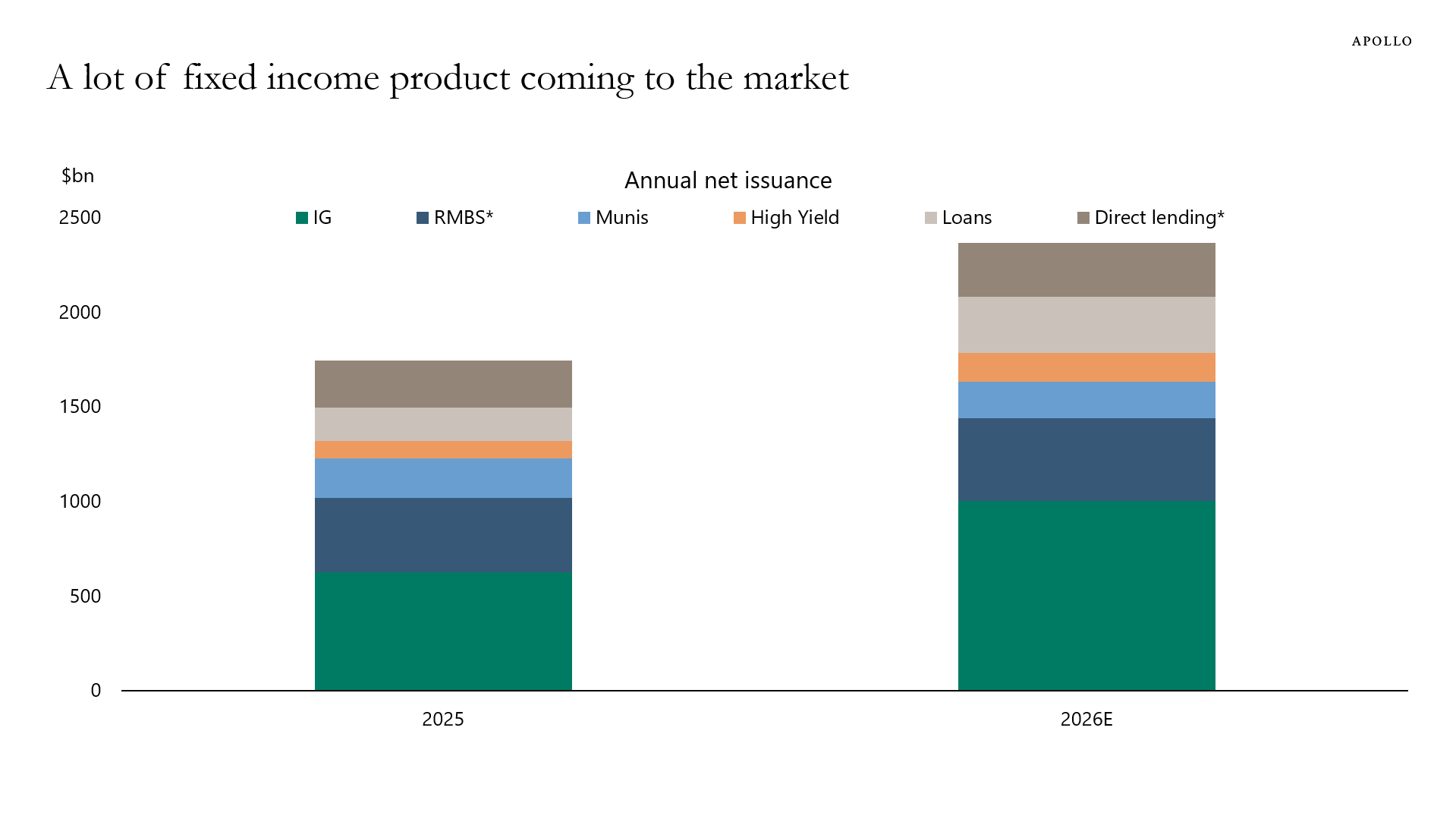
The components of this forecast do not perfectly align with the scope of the AI charts above. However, they describe an environment where hyperscaler bonds must compete with residential mortgage-backed securities (RMBS), municipal bonds, high-yield bonds, loans, and private credit for the same risk budget.
→ The market must not only find enough money to buy AI bonds; it must reserve enough capacity for a large, concentrated amount of duration risk that arrives just as system-wide supply is increasing.
Therefore, nominal value is only half the problem. The other half lies in the amount of interest-rate sensitivity that investors must actually bear.
2.2. DV01 shows concentration more clearly than notional
The market may still have enough money to buy bonds, but it no longer has enough budget to hold additional interest rate risk. This is where nominal issuance scale can be misleading.
Two bonds with the same face value do not create the same level of volatility. A 30- or 50-year bond is significantly more sensitive to interest rates than a 5-year bond. Therefore, one dollar of long-term debt may consume more risk budget than one dollar of short-term debt.
Technical note: DV01 is the metric used by the financial world to measure the change in a bond's value when yields shift by 1 basis point.
In the tracked index, six hyperscalers account for 5.4% of nominal value but 7.0% of DV01. When adding three semiconductor companies, the share increases to 7.1% in nominal terms and 8.8% in DV01.
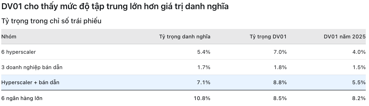
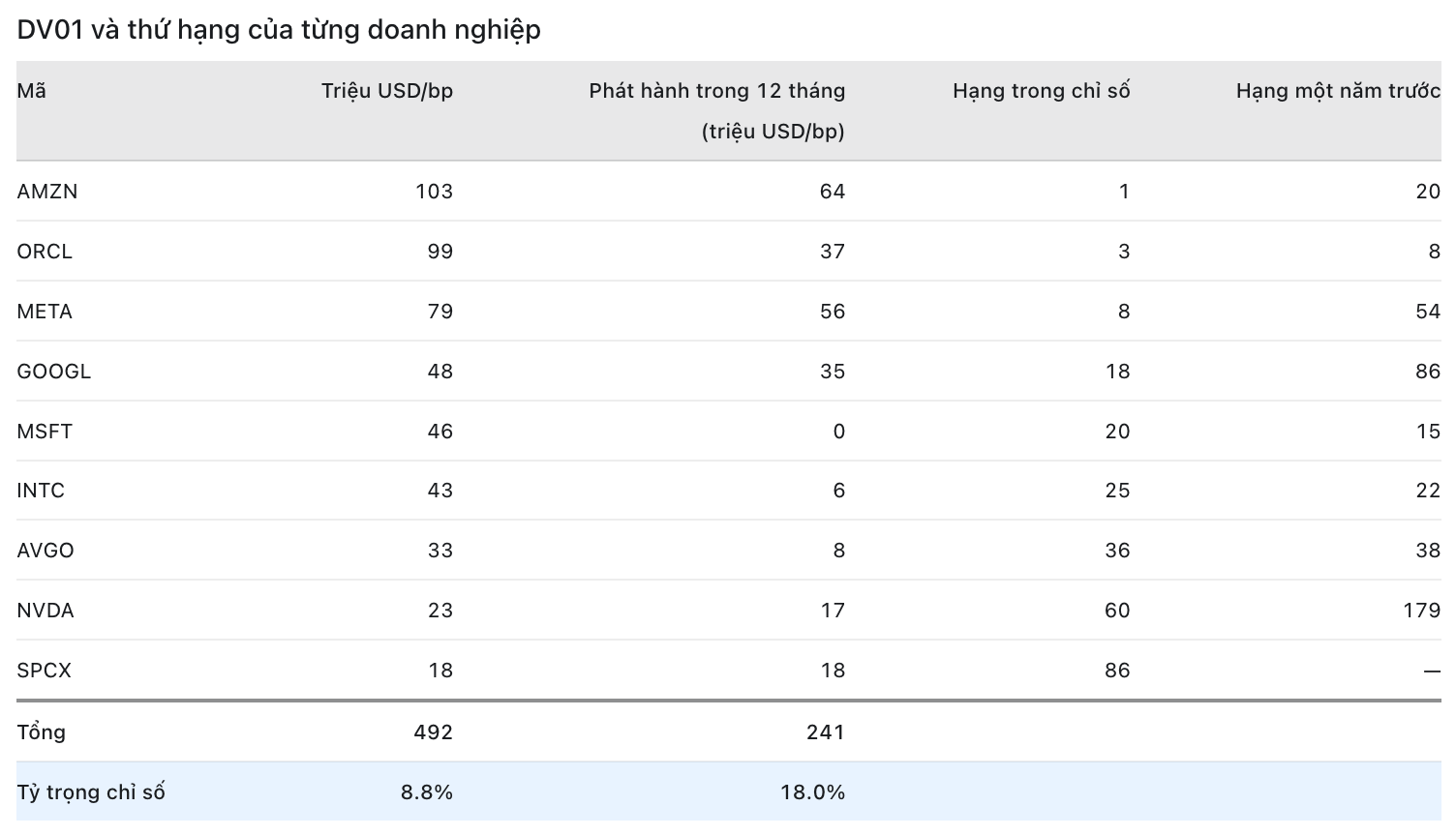
The rate of change is even more notable than the current concentration. Amazon has moved from 20th to 1st in DV01 in just one year; Oracle ranks 3rd, Meta 8th, and Alphabet has risen from 86th to 18th.
The total DV01 of the nine companies reached approximately $492 million per basis point. Nearly half-about $241 million-comes from bonds issued in the last 12 months, equivalent to nearly 18% of the new DV01 that the entire market must absorb.
It is necessary to distinguish between two layers of pressure:
Stock indicates how much risk the AI group currently occupies in the index.
Flow indicates how much they contribute to the risk just added to the market.
A portfolio manager may therefore still have cash but has already hit limits regarding interest rate sensitivity, price volatility, or sector concentration. In that case, new supply is only absorbed if the company pays a higher premium.
This pressure has begun to appear at the long end of the curve. The 10–30 year credit spread curve for A-rated or higher hyperscalers and Oracle is becoming steeper, while the curve for non-financial companies is flattening.
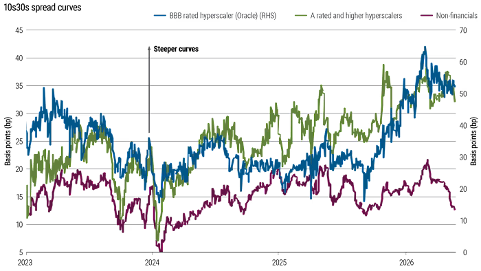
The slope here is calculated as the yield spread of 30-year bonds over Treasuries of the same maturity, minus the corresponding level for 10-year bonds. Therefore, a steeper curve does not necessarily mean all borrowing costs are rising; it shows that investors are demanding a larger premium to commit capital at the 30-year maturity.
Oracle is shown on a separate axis, so it cannot be directly compared in magnitude to the other two groups. The key information lies in the direction: the pressure is not just appearing at BBB issuers, but has spread to higher-rated hyperscalers as well.
→ The risk of AI supply does not lie solely in the amount of debt issued. A small group of companies is adding interest rate sensitivity so quickly that the market is beginning to price the capital locked in long-term maturities separately.
This is the pressure reflected in prices. To determine how much actual demand remains, we must look at the cover ratios of new deals.
2.3. Cover ratio is falling: excess demand is thinning
A bond deal may be sold out but still send a warning signal. What needs to be observed is how many orders investors place for every dollar of bonds offered.
Technical note - Cover ratio: Total value of orders placed divided by the size of the bond issuance. A higher ratio usually indicates stronger demand, but it can be inflated by orders placed in excess of actual needs.
The cover ratio for hyperscaler bond order books has fallen from nearly 5x in February 2026 to about 2.8x in March, 2.7x in May, and below 2x in July. During the same period, the average for the broader IG market remained above 3x.
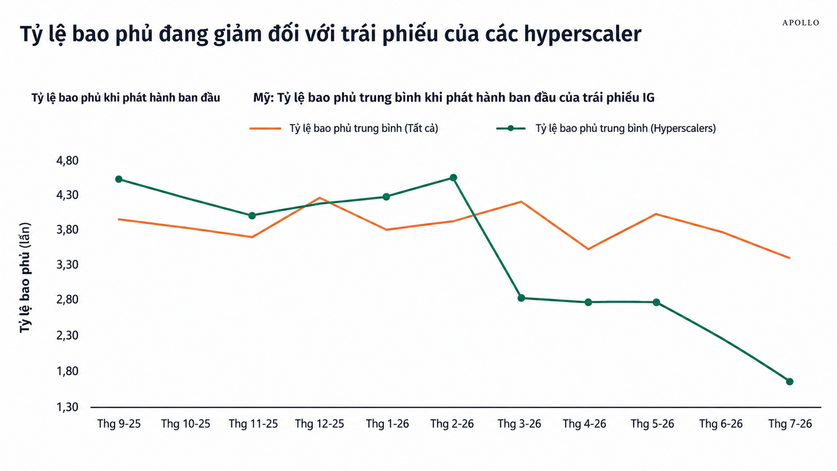
A level below 2x still means that orders exceed the issuance size. The market has not closed. But the layer of excess demand has thinned, giving companies less ability to tighten yield spreads at the last minute and potentially forcing them to pay a higher concession to complete the deal.
One should not read a single ratio as a verdict on credit quality. The cover ratio also depends on:
the size and maturity of the deal;
whether the initial price is attractive enough;
market conditions on the day of issuance;
how the underwriter manages the order book.
What is noteworthy is that the direction of the data coincides with the increase in supply and DV01. Investors are not withdrawing from the big tech group, but they are becoming more price-sensitive.
→ The current signal is not a lack of buyers, but that buyers no longer accept every price just because the company name is strong enough.
When demand becomes conditional, secondary market yield spreads are where the new premium is more clearly reflected.
2.4 Yield spreads are widening: the market is repricing the entire group
A successfully distributed deal does not mean the pressure has disappeared. As a continuous volume of new bonds enters portfolios, the risk that investors do not want to hold will gradually be reflected in secondary market prices.
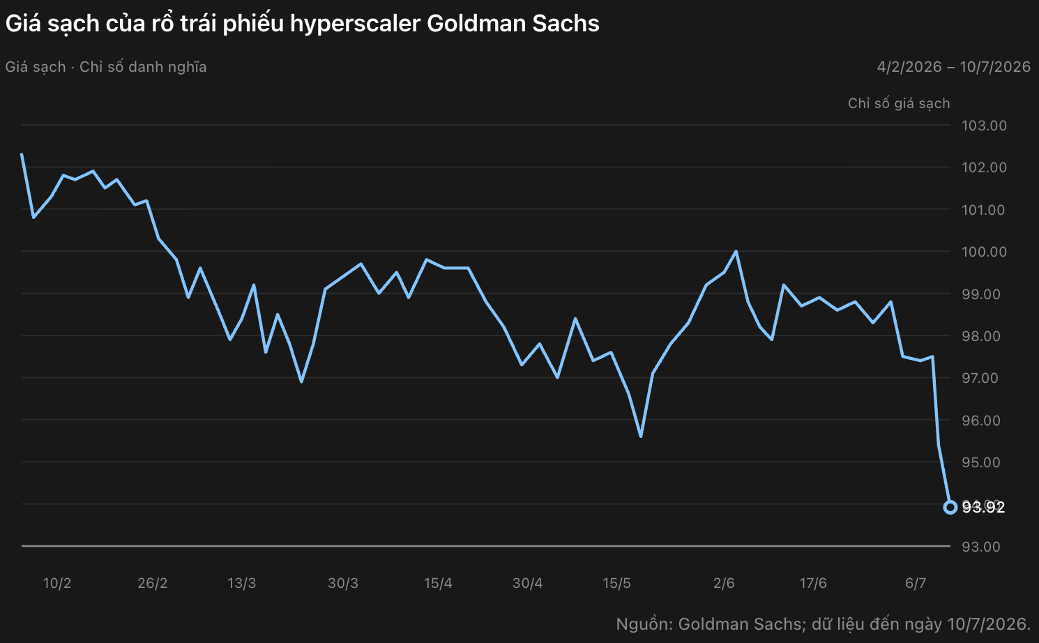
The clean price of the GSUCHS30 hyperscaler bond basket fell to 93.92 points on July 10, 2026. This trend is not a pure measure of credit risk, as bond prices are also affected by interest rates and do not include accrued interest. However, it shows that absorption pressure has shifted from the issuance order book to the actual performance of the portfolio.
Clean price is the bond price excluding the coupon interest accrued since the last payment period.
The weakness stems from more than just Treasury rate volatility. Spreads for both the A-rated and above hyperscaler group and the BBB group have widened relative to the U.S. investment-grade (IG) corporate index. This indicates that the repricing has spread across multiple credit quality tiers, rather than being concentrated entirely on a single issuer.
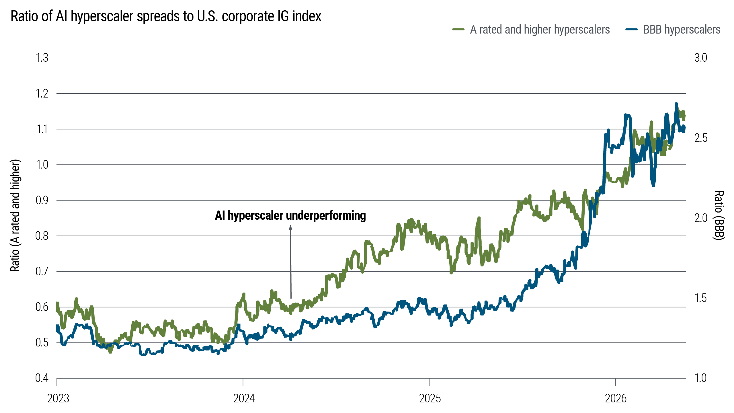
The two groups are plotted on separate axes, so the absolute levels of the two lines cannot be directly compared.
✵✵✵ The key takeaway lies in the trajectory: both high-quality issuers and the BBB group are trading less favorably compared to their respective IG benchmarks.
The divergence in magnitude remains significant. The higher-rated group holds more cash, has greater operating cash flow (CFO) generation capacity, and better leverage headroom. The BBB group is more sensitive to weakening free cash flow (FCF), refinancing costs, and the ability to issue additional debt. The market is therefore pricing in two types of risks simultaneously:
General group risks: rising supply, longer maturities, and increasing concentration within the index.
Issuer-specific risks: balance sheet quality, the timing of FCF recovery, and reliance on external capital.
This is not yet a signal that the market doubts the solvency of the entire group. Hyperscalers still have access to capital and largely maintain strong credit foundations. What has changed is that investors no longer view Big Tech debt as a supply that can be expanded almost indefinitely without requiring an additional risk premium.
→ The market has not refused to fund the AI race; it is forcing each issuer to pay a price that accurately reflects the duration, supply, and cash flow certainty they are introducing into the system.
Bond prices and relative spreads confirm that the repricing process has begun. To determine whether this pressure is primarily driven by supply and demand or has evolved into genuine credit concerns, one must look to CDS.
2.5. CDS confirms the shift from oversupply to credit selectivity
Five-year credit default swaps (CDS) for the Big Tech group have also widened, even though they are not directly impacted by interest rate sensitivity like cash bonds. The basket of Amazon, Google, Apple, and Microsoft moved from the 20–25 basis point range to approximately 45–47 basis points; when Oracle is added, the CDS approaches 70–75 basis points.
Technical note - Hyperscaler CDS: The cost of insuring against a hyperscaler default, typically quoted in basis points per year. Rising CDS indicates that the market is demanding a higher credit risk premium, but it does not mean the company is on the verge of default.
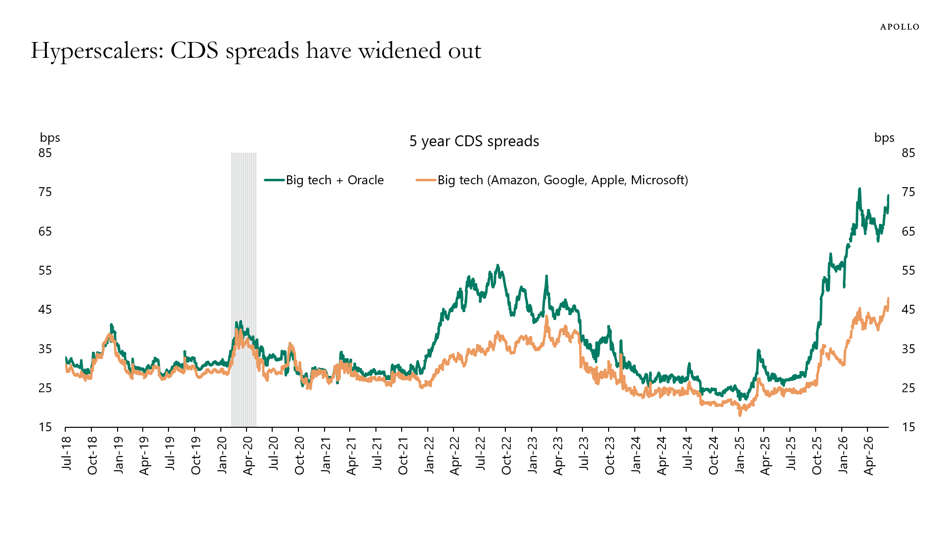
CDS is still influenced by liquidity, hedging demand, and basket structure. However, the fact that both cash bonds and CDS are widening suggests the market no longer views this as merely a technical story of interest rate sensitivity.
The progression can be divided into three states:
Temporary oversupply: coverage ratios decline and concessions increase, but CDS and FCF forecasts remain largely stable.
Selective funding: lower coverage ratios, widening bond yield spreads and CDS, but the market remains open to companies and projects with strong fundamentals.
Credit deterioration: CDS continues to rise while FCF is downgraded, leverage worsens, and multiple funding channels tighten simultaneously.
Current data best fits the second state. Investors are still willing to provide capital, but they are beginning to distinguish more clearly between corporate reputation, project quality, and the timing of cash flow generation.
→ The credit market has not voted against AI; it is abandoning the assumption that every AI investment deserves to be funded at the same price.
This selectivity brings the problem back to the decisive variable: whether free cash flow will recover soon enough.
PART III - THE DECISIVE PROBLEM IS THE TIMING OF CASH FLOW
3.1. Profits remain strong, but investment intensity has surpassed the dot-com era
Comparing the current period to the late 1990s easily leads to two extreme conclusions: either AI is a bubble identical to the dot-com era, or strong profit foundations make all concerns meaningless. The reality lies between these two views.
The similarity lies in investment intensity. The share of technology investment in GDP has surpassed the peak of the late 1990s and has risen sharply in recent months. The economy is deploying a massive amount of capital before knowing for certain how effectively the new capacity will be utilized.
The difference lies in the starting point. During the dot-com cycle, profit margins on macroeconomic measures peaked in late 1997, years before the bubble burst. Currently, corporate profits remain near record levels and profit expectations continue to be revised upward.
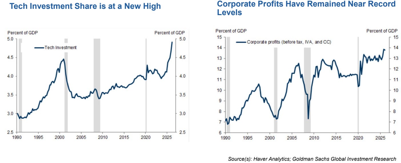
This foundation reduces the probability of a 2000-style collapse in the short term. Companies are not building on a weakened profit machine; they are using significant cash flow from current operations to fund a new opportunity.
But strong profits also come with high expectations. The gap between S&P 500 12-month forward earnings and cyclically adjusted earnings has reached a multi-year high.
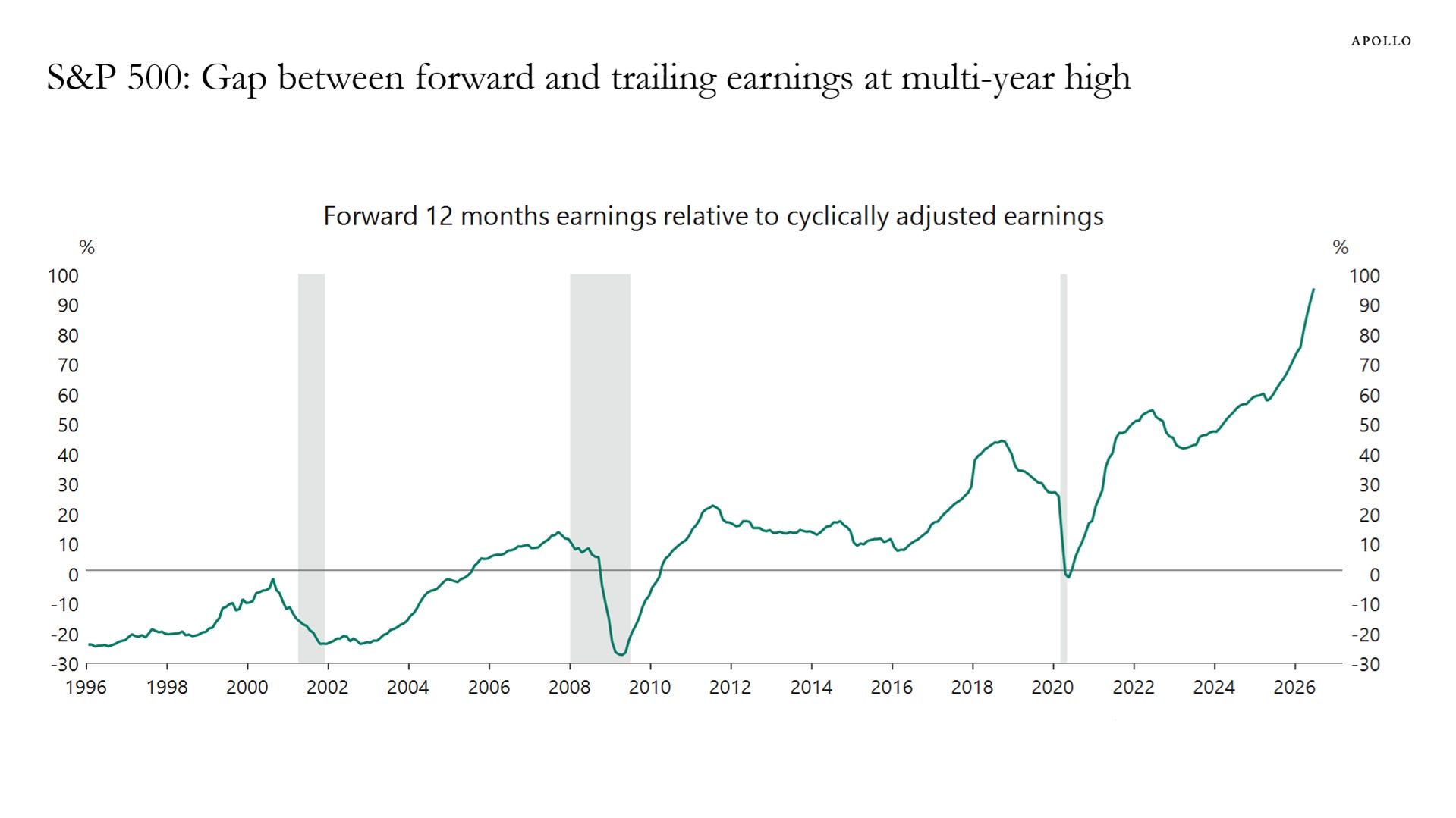
A gap of nearly 100% does not mean the market forecasts a 100% increase in profits in one year. It reflects the difference between two measurement methods, but it still shows that asset prices are increasingly dependent on a future that is better than the present.
The remaining issue is that market-wide profits do not mean AI capital has generated commensurate returns. Corporate profits may continue to hit peaks while hyperscaler FCF declines, because capex is spent immediately while revenue from new capacity takes time to materialize.
→ The current cycle has a better profit foundation than the dot-com era, but it also sets a higher return standard because both capital volume and expectations have risen significantly.
Therefore, the decisive question is not whether the economy is currently profitable. The question is whether cash flow will emerge at the right companies and at the right time to fund the capital being deployed.
3.2. Forecasted FCF has reflected the capex shock
The health of the income statement can mask the pressure building in the cash flow statement. Cloud revenue is still growing, backlogs remain large, and balance sheets are still strong, but the cash remaining after investment has declined rapidly.
Total 12-month forecasted free cash flow (FCF) for the five hyperscalers approached $300 billion in 2024, then declined sharply in 2025–2026. Oracle turns negative at the end of the forecast series.
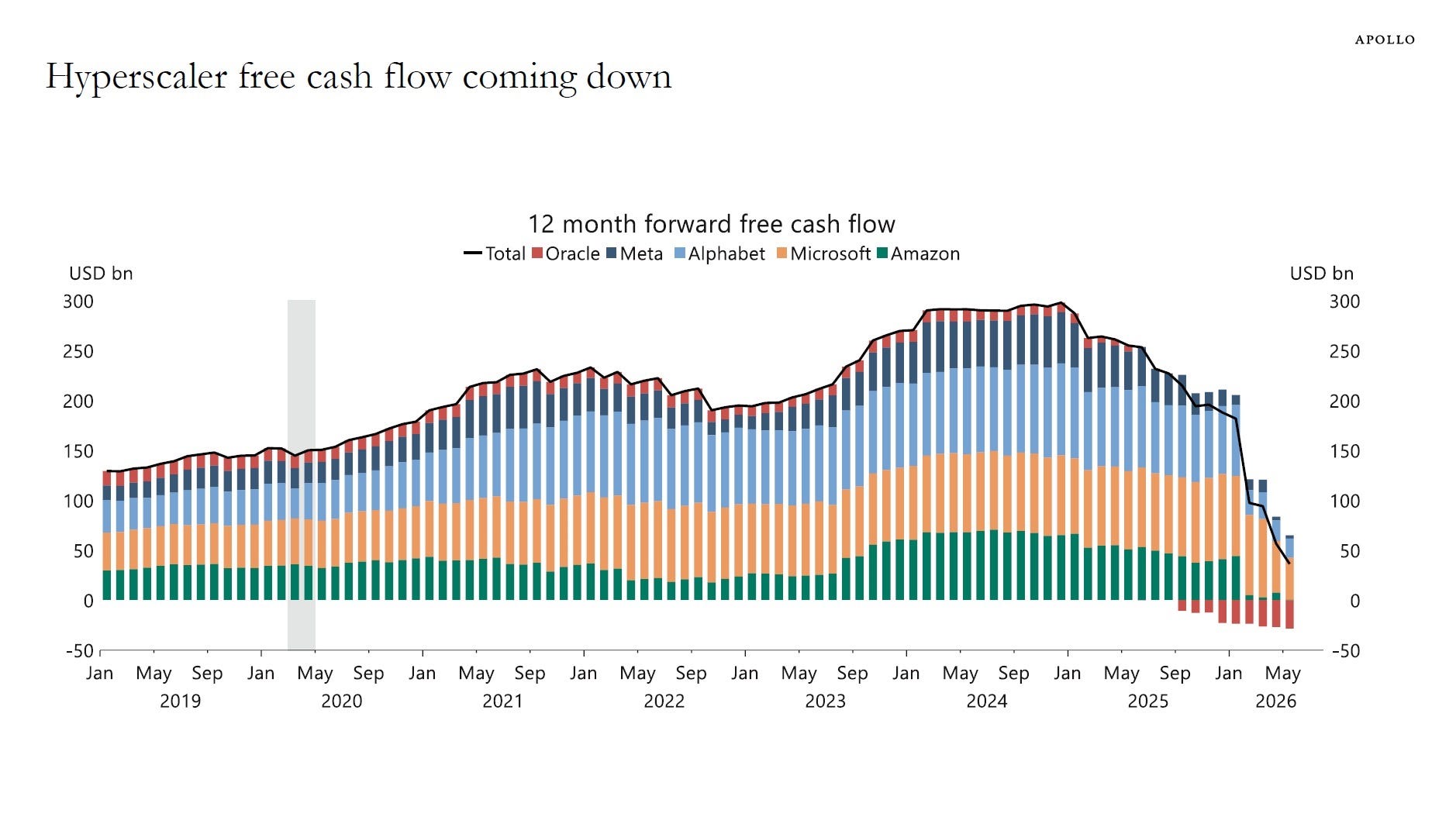
This trend does not necessarily indicate that core operations are weakening. Most of the pressure comes from capex growing faster than CFO. However, for creditors, the cause does not change the consequence: the amount of cash available for self-funding, share buybacks, and liquidity protection has shrunk.
When FCF is compressed, companies have four main options:
issue more bonds or borrow from banks;
increase the use of leases and project financing;
reduce share buybacks or non-core investments;
accept using more of the cash accumulated on the balance sheet.
Each option allocates risk in a different way. Issuing debt directly increases leverage; leases create fixed obligations; reducing share buybacks protects credit but may pressure valuations; and using cash reduces the buffer for future years.
→ The capex shock has appeared in FCF before fully appearing in leverage ratios.
What the market is pricing is not one year of low cash flow, but the length of the period before FCF returns.
3.3. Consensus forecasts bet on a major rebound from 2028
The market's base case does not assume FCF will continue to decline indefinitely. It bets that the assets currently being built will transition from cash-consuming to cash-generating within a few years.
Forecasts expect FCF for the four major hyperscalers to begin a strong recovery from 2028 and exceed $450 billion by 2030.
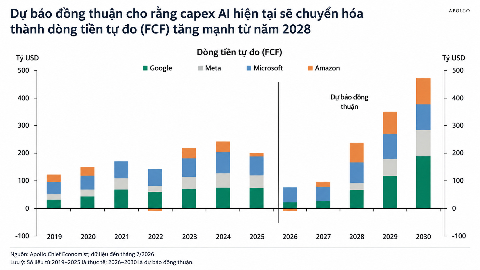
This story consists of three steps:
Capex increases sharply and compresses FCF in 2026–2027.
New capacity is filled as businesses adopt AI more broadly and inference demand increases.
Capex growth rates normalize while revenue continues to expand, helping FCF rebound.
That path is entirely possible. But this is not just a forecast of profit scale; it is also a forecast of timing. A project with good economic value over 10 years can still create credit pressure if it must be refinanced twice before generating sufficient cash.
The gap between market-expected earnings and actual earnings in the event of slower AI deployment illustrates this very risk. The gap is a space for repricing, not a forecast of losses or default.
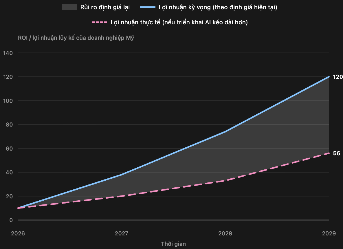
If the FCF rebound is delayed by one or two years, the long-term value of AI may remain unchanged, but the capital requirement in the interim will be greater. In that case:
debt and leases continue to rise before cash flow recovers;
interest expenses and fixed obligations accumulate further;
leverage worsens because the numerator increases before the denominator;
the market demands a higher premium for the next issuance.
→ For shareholders, delayed returns may be a valuation issue; for creditors, it is a funding gap that must be filled with real cash.
Therefore, 2028 is not just a milestone in a forecast model. It is the point where the AI story must begin to self-fund better to prevent credit pressure from continuing to accumulate.
3.4. Lower computing costs do not guarantee higher profit margins
The most positive argument for FCF lies in the economies of scale of each token. If hardware and inference costs continue to fall while selling prices hold steady, profit margins could expand rapidly once capacity reaches sufficient utilization.
Computing costs on GPU, TPU, AMD, and Trainium platforms are forecast to continue falling, while output token prices for leading models are more stable. This gap creates the potential for margin improvement from the first half of 2026.
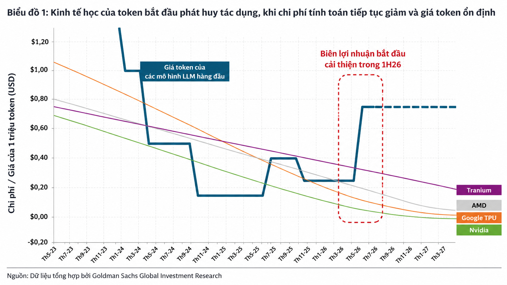
However, lower unit costs only become FCF when companies retain the savings. This depends on three variables:
Price: Does competition force suppliers to pass on all cost benefits to customers?
Volume: Does a cheaper token generate enough new demand to offset the lower price per unit?
Compute intensity: Do better models consume so many resources that they negate hardware advancements?
Subscription models, advertising, per-user fees, or direct integration into business workflows may help retain value better than pure token sales. Conversely, open-source competition and low pricing could drive a surge in usage that outpaces revenue growth per unit of compute.
→ Cost reduction is a necessary condition for monetization, but usage levels, pricing power, and revenue per unit of compute determine FCF.
Even as unit economics improve, another pressure is quietly shifting from the balance sheet to the income statement: depreciation.
3.5. The wall of depreciation will follow the cash shock.
Capex impacts FCF as soon as cash is spent, but it does not flow directly into the income statement as an expense. During the construction phase, assets are recorded as construction-in-progress; depreciation only begins once capacity is put into service.
This lag means current profit margins may underestimate the cost burden of coming years. Oracle's depreciation-to-revenue ratio is projected to rise from approximately 7% to 28% by fiscal year 2028, while Meta's is expected to climb from 9% to 19%. Microsoft and Google are following a similar trajectory.
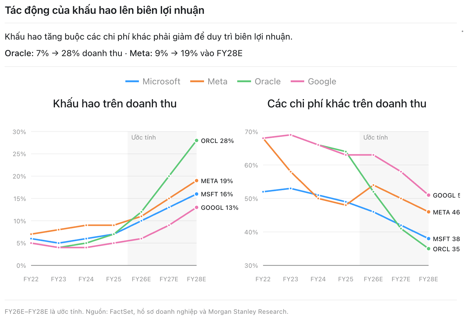
As depreciation accounts for a larger share, other expenses must decrease or revenue must be adjusted upward if the company intends to maintain margins. This is a difficult requirement when capacity is underutilized or competition limits pricing power.
It is necessary to distinguish clearly between accounting impact and cash impact:
depreciation is a non-cash expense and is added back in CFO;
it does not directly reduce FCF a second time after capex has been spent;
however, it reduces EBIT, affecting profit-based interest coverage and revealing the scale of assets requiring maintenance;
short chip lifecycles can lead to faster depreciation, impairment, or higher-than-expected replacement investment needs.
Credit risk only intensifies when three pressures converge: rising depreciation, sustained high capex, and lagging revenue from new capacity. In such a scenario, accounting margins compress while cash continues to be absorbed into the next investment cycle.
→ The capex shock appears first in FCF; the depreciation wall appears later in earnings. The gap between these two points does not eliminate the cost; it merely delays the moment it becomes fully visible.
Recorded assets do not yet represent the full economic commitment. A significant portion of the build-out resides in leases, purchase obligations, and supplier balance sheets.
PART IV - LEVERAGE DOES NOT DISAPPEAR, IT CHANGES ADDRESS
4.1. Public bonds are only the most visible layer of capital
Hyperscaler bond debt has grown rapidly, but remains small relative to their market capitalization. The five major companies have approximately $384 billion in index-eligible debt, equivalent to nearly 4% of the IG market, while accounting for about 20% of the S&P 500's market cap.
This discrepancy can create the impression that balance sheets have plenty of room. That is true at the corporate level, but not yet at the systemic level. The AI build-out is financed through multiple layers, each shifting risk to a different group of investors.
The primary capital layers include:
hyperscaler CFO and equity;
public bonds and bank loans;
project financing via special purpose vehicles (SPVs), asset-backed securities (ABS), and commercial mortgage-backed securities (CMBS) tied to data centers;
leases, purchase obligations, and capacity commitments;
private credit or vendor financing in downstream links.
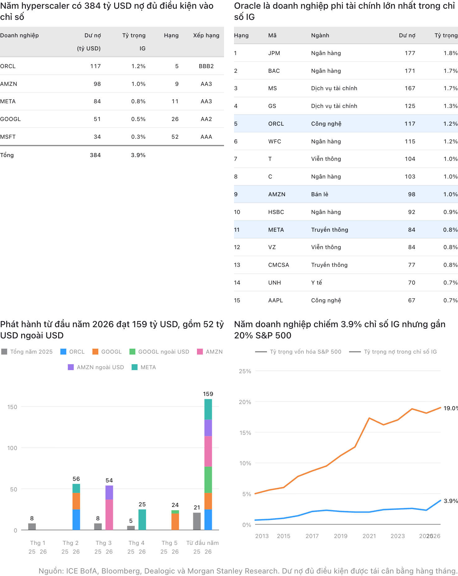
Structuring this fragmentation may be economically sound. Specific assets are matched with specific cash flows; companies retain flexibility; lenders have rights to the project rather than the entire group.
But allocation does not mean elimination. Each layer of financing remains directly or indirectly dependent on AI demand, capacity utilization, and the quality of end-customer commitments.
→ Hyperscaler bonds are the most measurable part of the capital cycle, not the total amount of leverage the build-out has created.
To assess true risk, one must trace obligations to the final balance sheet that must bear them.
4.2. Off-balance-sheet commitments shift leverage to suppliers
Moving an obligation off a hyperscaler's balance sheet does not make the economic debt disappear. It only changes where the debt is recorded and who must refinance if AI revenue arrives late.
The relevant companies have signed approximately $982 billion in purchase obligations and $822 billion in future leases. These are multi-year commitments that may overlap and cannot be added directly to annual capex. Nevertheless, their scale indicates that the amount promised to be spent is significantly larger than what appears in reported debt.
Accounting-wise, purchase obligations typically only become payables when goods or services are delivered. Signed leases also generally do not create right-of-use assets and lease liabilities before the commencement date. Information may be in the footnotes, but it does not enter reported leverage like bonds or loans.
Obligations not recorded at the hyperscaler can still create debt elsewhere:
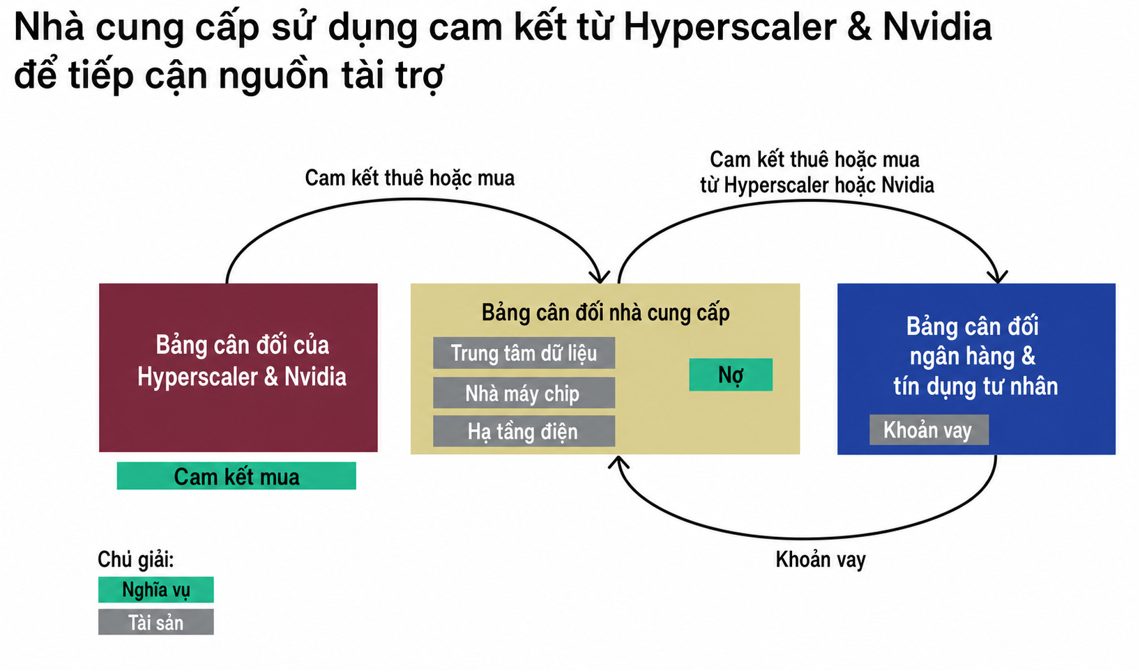
A hyperscaler or Nvidia signs long-term lease, chip purchase, power, or capacity contracts with a supplier.
The supplier uses the contract-backed cash flow to support the construction of data centers, fabs, or power infrastructure.
Banks and private credit funds provide financing; the loan is recorded on the supplier's balance sheet.
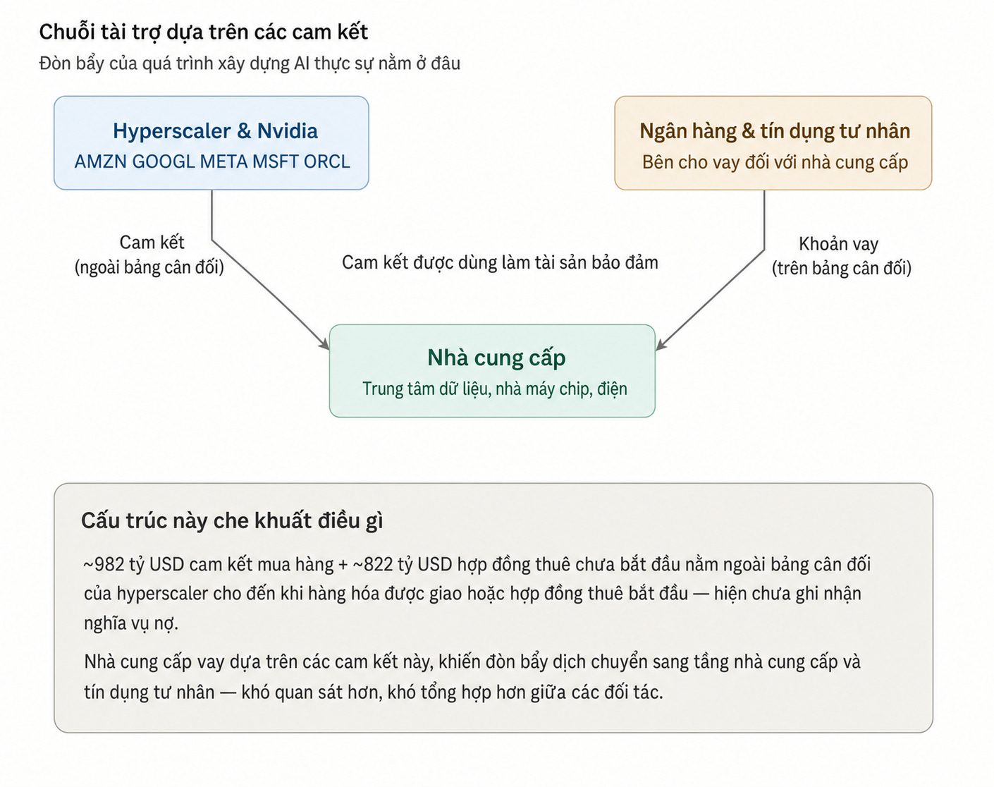
Not every contract is formally collateralized. Depending on the structure, lenders may receive rights to the contract or simply use projected revenue streams during due diligence. The common thread is that the hyperscaler's credit quality enhances the partner's borrowing capacity.
Actual relationships are even more intertwined than a three-party model. A company can simultaneously play multiple roles:
customer purchasing capacity;
shareholder of the supplier;
revenue-sharing partner;
provider of preferential financing;
guarantor of output or participant in repurchase agreements.
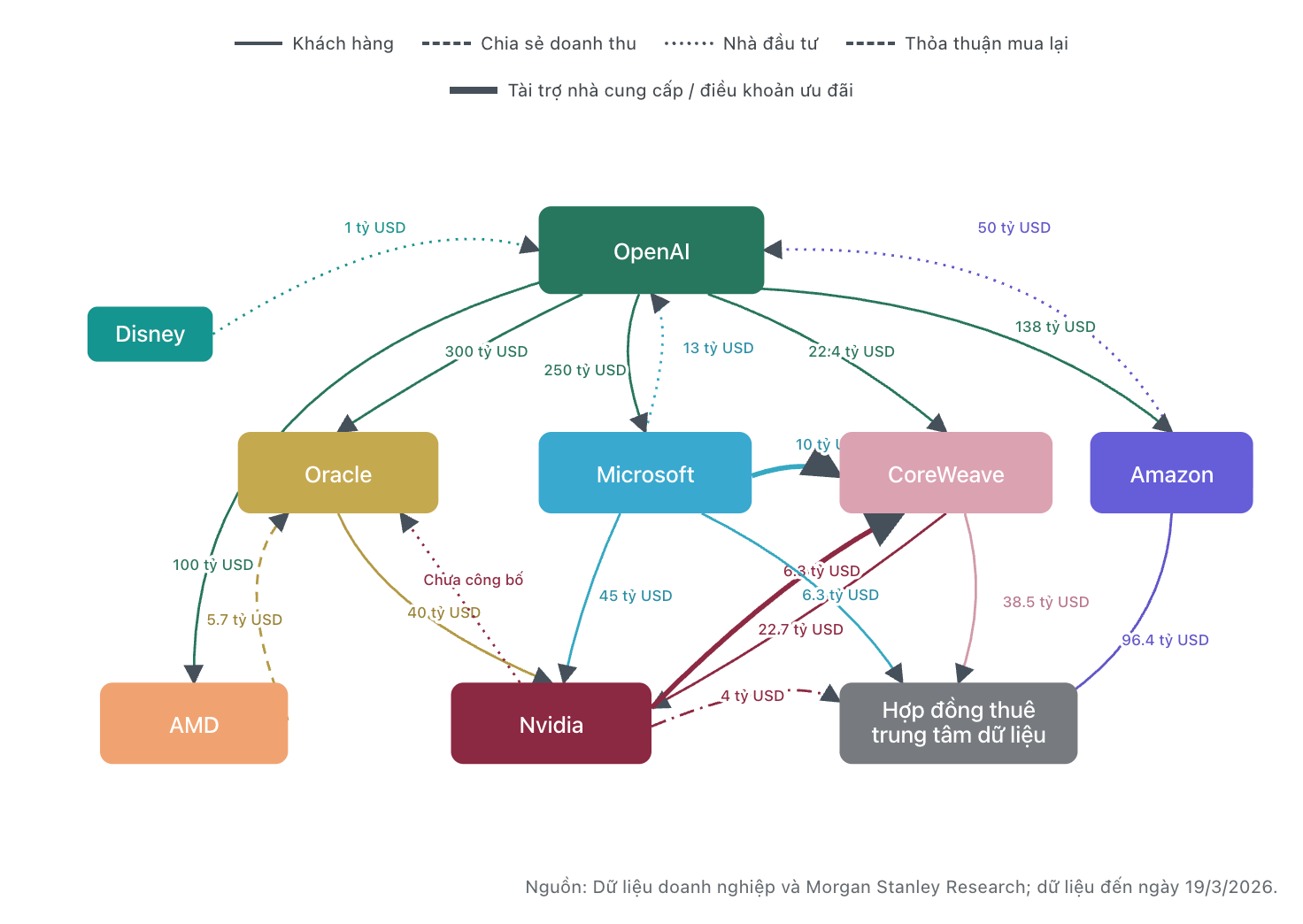
This structure may allocate capital more efficiently, but it makes the level of exposure difficult to aggregate. A hyperscaler may lease capacity, invest in that very partner, and simultaneously generate revenue streams that help the partner borrow more. Risk, in that case, does not rest entirely on any single balance sheet.
Remaining Performance Obligations (RPO) for Microsoft, Oracle, Amazon, Google, and CoreWeave have grown from approximately $568 billion to over $2.1 trillion, indicating that the volume of contracted activity has expanded very rapidly.
Technical note - Remaining Performance Obligations (RPO) is the value of revenue that has been contracted but not yet recognized because goods or services have not been fully provided. RPO reflects future contract revenue, not cash collected or customer debt.
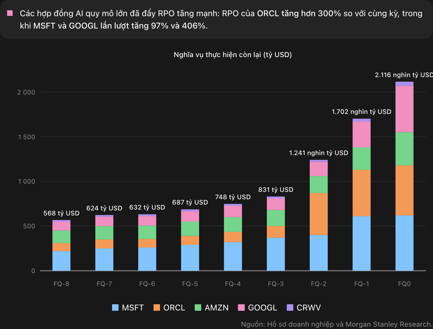
RPO is revenue that has been signed but not yet fully recognized by the supplier. It is not customer debt, may overlap with other contractual relationships, and is not added directly to purchase or lease obligations. The value of the metric lies in showing that contract-based cash flows are large enough to serve as a foundation for due diligence on many new projects.
The structure only becomes dangerous when the obligation schedule runs faster than the revenue generation schedule. If utilization is low, the supplier must still pay interest and complete the project; the hyperscaler may still have to fulfill minimum purchase clauses, long-term leases, or mandatory payments. When refinancing costs rise, the project may require more equity, relaxed covenants, or support from sponsors.
→ Off-balance-sheet does not mean off-risk. Leverage still exists; it just resides with suppliers, banks, or private credit funds instead of where investors usually look first.
Therefore, the critical question is not whether an obligation is called debt, a lease, or RPO. The question is which balance sheet must continue to pay if AI cash flows do not appear on schedule.
4.3. The ultimate risk lies where refinancing must occur
In a favorable scenario, the multi-layered structure helps capital reach the right assets and the right investors. Capacity is filled, contract-based cash flows service project debt, and hyperscalers retain room for subsequent technology generations.
In an unfavorable scenario, that same structure makes the shock harder to observe. A project may begin to face pressure at the SPV level, then spread to private credit funds, bridge loans, ABS, or CMBS before appearing on the hyperscaler's balance sheet.
Investors must therefore monitor obligations beyond reported debt:
current leases and contracts signed but not yet commenced;
purchase obligations, minimum purchase clauses, and capacity commitments;
guarantees, liquidity support, and recourse rights against sponsors;
exposure to partners where the company is both a customer and a shareholder.
Aggregation must avoid two opposing errors. Ignoring off-balance-sheet obligations will underestimate risk; mechanically adding every number together will create a false total because contracts may overlap, cancel out, or belong to different years.
→ The correct unit of analysis is no longer an individual company, but the entire chain of contracts connecting capacity buyers, asset owners, and capital providers.
Only by knowing where loans must be rolled over, who owns the assets, and who has the ultimate obligation to pay, can investors see the full leverage of the AI cycle.
PART V - KOSPI IS AN AMPLIFIER, NOT A CAUSE
A sell-off in South Korea is easily read as the market's verdict on the AI cycle. But the KOSPI does not determine hyperscaler budgets, nor does it directly decide how many data centers will be built. It sits at the downstream end of the investment chain, where small changes in order expectations can create much larger fluctuations in stock prices.
Therefore, the KOSPI has value as an early signal. It shows that investors are changing how they value the hardware cycle, but it does not in itself prove that AI demand, cash flow, or financing capacity has weakened.
5.1. Why signals often appear early in Korea
If hyperscalers are where capex is decided, Korea is one of the places that reflects early expectations regarding the volume of hardware to be ordered. This market is home to many memory, HBM, semiconductor equipment, and component companies located near the center of the AI supply chain.
That sensitivity stems from business structure. A hyperscaler can offset an AI slowdown with advertising, software, e-commerce, or traditional cloud services. Memory suppliers are more directly dependent on the output, pricing, and capacity expansion plans of a few large customers.
The investor structure causes price reactions to appear even earlier than corporate data. Cumulative capital flows during the 2025–2026 period show that foreign investors have net sold over $100 billion in Korean stocks, while domestic retail and institutional investors have become the primary absorbing force.
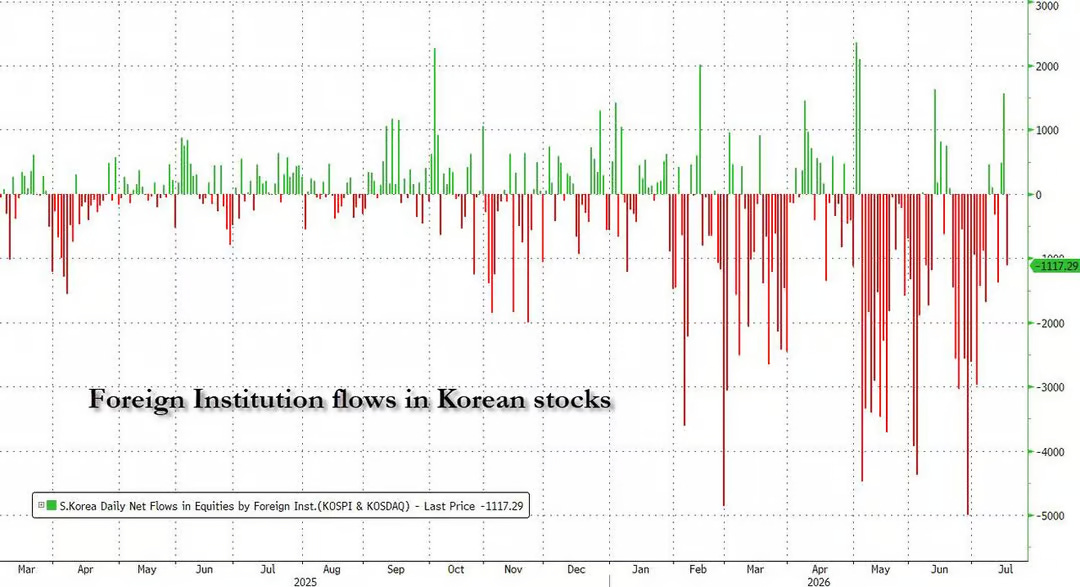
This development is important not because foreign capital always correctly predicts the cycle, but because it shows that prices can change sharply before actual orders are adjusted. Global investors often use Korea as a highly liquid tool to trade expectations on semiconductors, Asia, and tech growth.
Three characteristics cause signals here to appear early:
earnings are concentrated in memory and the semiconductor cycle;
revenue is highly dependent on the purchasing plans of a small group of large customers;
the position of foreign investors can be reduced rapidly when the USD and volatility rise together.
→ The KOSPI does not generate AI credit risk; it is typically where the market adjusts expectations for capex and orders before changes appear in corporate earnings reports.
Therefore, a decline in South Korea is worth monitoring, but it is not yet sufficient to conclude that the AI cycle has broken.
5.2. Market leverage can turn a correction into a sell-off
The speed of a price decline does not necessarily reflect an equivalent level of weakness in actual demand. ETFs, trend-following strategies, margin trading, options, and volatility-control funds can all transform an initial shift in expectations into a mechanical deleveraging process.
The current volatility shows that amplification mechanisms have been operating at a scale rarely seen. The 30-day volatility of the KOSPI has risen to 81.95, the highest level in the entire data series dating back to 1980.
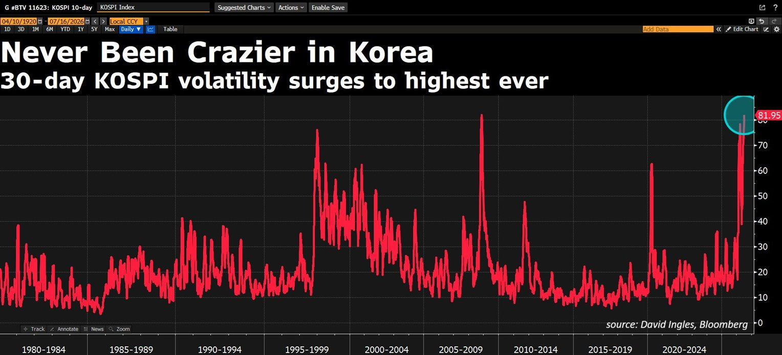
This figure measures the speed of price movement, not the cause of the shock. Volatility can rise because profit prospects deteriorate, but it can also rise due to concentrated positioning, declining liquidity, and simultaneous hedging activity.
Margin data helps explain the underlying mechanism. Brokerage margin debt has risen sharply, while the ratio of margin calls to outstanding debt has also seen sudden spikes. As stock prices fall, collateral loses value, forcing investors to either add cash or reduce positions.
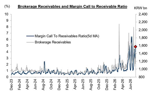
The amplification process typically follows a short sequence:
falling prices trigger margin calls;
rising volatility causes funds to reduce risk limits;
trend-following strategies and options hedging generate additional sell orders;
foreign capital outflows weaken liquidity just as selling demand increases.
Leverage here is different from corporate debt. It lies in how assets are held and in the rules that force investors to react when prices change.
→ Market leverage makes prices move faster than fundamental data; therefore, a heavy sell-off cannot yet be seen as proof that AI demand has weakened to the same extent.
However, volatility will be more concerning if it lasts long enough to affect companies' ability to raise capital and their investment decisions.
5.3. Supply chain sensitivity is always higher than that of hyperscalers
Hyperscalers and suppliers are both exposed to the AI cycle, but their profit structures are very different. Hyperscalers own multiple revenue streams, while memory or semiconductor equipment manufacturers often have high fixed costs and are more directly dependent on a few product lines.
The strongest reactions typically appear in:
memory and HBM;
advanced packaging and semiconductor equipment;
optical networking and connectivity components;
data centers, cooling systems, and power infrastructure.
When orders increase, fixed costs are spread over higher output, and profits can grow faster than revenue. The same mechanism operates in reverse: if the growth rate of orders is slower than expected, future margins can be sharply adjusted even if revenue continues to grow.
Therefore, the market does not need to wait for hyperscalers to officially cut capex. Supplier stock prices can fall as soon as investors forecast rising inventories, HBM prices peaking, or capacity expansion slowing down.
→ Financial leverage accelerates the speed of selling, while operating leverage increases the magnitude of profit changes. When these two factors meet, the KOSPI can react more strongly than the initial fundamental shock.
But amplification does not mean confirmation. Stock prices reflect expectations; orders and financing conditions indicate whether those expectations are becoming reality.
5.4. When the KOSPI becomes a macro signal
A single sell-off could reflect profit-taking, a strong USD, geopolitical tension, or technical deleveraging. It only becomes evidence of an AI shock when independent markets begin to transmit the same message.
The confirmation process can be divided into three layers:
Market prices: semiconductor stocks fall, foreign capital exits, and volatility remains high.
Financing conditions: yield spreads and CDS of hyperscalers continue to widen, coverage ratios fall, new issuance concessions increase, and banks become more cautious with new projects.
Fundamental data: FCF forecasts are lowered, leverage increases, capex guidance weakens, and orders for HBM, optical networking, data centers, or power are cut.
If only the first layer deteriorates, the development is likely still a deleveraging event in the capital market. If the second layer also weakens, the shock begins to affect the cost of capital. When all three layers shift simultaneously, volatility in South Korea is no longer just an early signal; it becomes a link in the process of investment contraction.
→ The KOSPI detects changes in expectations; the credit market and order data determine whether that is noise or a turning point in the cycle.
This boundary is particularly important because an asset shock only becomes an economic shock when it causes companies to change their investment behavior.
PART VI - FROM CREDIT CONCERNS TO MACRO SHOCK
6.1. Three paths of the AI cycle
Large capex does not automatically lead to a crisis. The same data center systems, chips, and power infrastructure being built today could produce three completely different outcomes, depending on the speed at which new capacity is utilized and converted into cash flow.
Scenario 1: Cash flow catches up with investment
Demand for AI inference and enterprise applications grows fast enough to fill new capacity. Computing costs fall, revenue expands, and FCF begins to recover from 2027–2028. Leverage peaks before gradually declining.
In this case, yield spreads may remain higher than before due to the large volume of bonds issued, but the market continues to absorb the supply. Credit pressure stems primarily from temporary supply-demand imbalances, not from weakened debt-servicing capacity.
Scenario 2: Technology is right, but cash flow arrives late
AI eventually creates economic value, but the deployment process takes longer than expected. Capacity is not fully utilized while depreciation, rent, electricity costs, and interest expenses have already begun to rise. To maintain their competitive position, companies must continue to invest before old projects generate enough cash.
Capital does not disappear, but it becomes more selective:
Companies with strong balance sheets can still issue bonds.
Projects with long-term contracts and clear cash flows are still funded.
Weaker structures must pay higher interest rates, add equity, or delay implementation.
This is the stage where the long-term value of AI has not been denied, but the market begins to question the ability to fund the waiting period.
Scenario 3: Funding limits force companies to cut capex
The bad scenario only forms when FCF continues to be lowered while the bond market, banks, and private credit simultaneously tighten conditions. The cost of capital then rises enough that some projects no longer meet the required rate of return.
Hyperscalers are forced to postpone or cut investment. The subsequent impact cascades down to memory, semiconductor equipment, optical networking, data centers, and power infrastructure. The fluctuations in the KOSPI then no longer just reflect investors reducing positions, but begin to signal the weakening of real investment.
→ The boundary between the three scenarios does not lie in whether AI is useful or not. It lies in whether cash flow arrives before funding becomes too expensive.
Current data is most consistent with the second scenario: investment continues, but the market increasingly demands clearer evidence of the payback period.
6.2. Monitoring dashboard: from supply to project economics
No single indicator can determine which path the cycle is following. Yield spreads can rise because of supply; FCF can fall because companies are actively investing; the KOSPI can plunge because investors are deleveraging.
Signals are only truly reliable when three layers of data move together.
Layer one: Is the market still willing to provide capital?
OAS compared to the broader IG market indicates whether AI bonds are being repriced more heavily than the rest.
New issuance concessions measure the additional yield companies must pay to attract buyers.
Coverage ratios and order book quality reflect the true depth of demand.
Post-issuance trading prices indicate whether bonds have been sustainably distributed or only sold out due to attractive pricing.
New DV01 measures the amount of interest rate risk the market must absorb, rather than just looking at the face value of the issuance.
Layer two: Can companies self-fund their investments?
Projected FCF and the capex/CFO ratio show how much operating cash flow is being absorbed by investment.
Capacity utilization and revenue per unit of compute show whether new infrastructure is actually generating cash.
Depreciation and fixed obligations reflect the portion of costs that will gradually flow into earnings.
Leverage after lease adjustments shows a fuller financial burden than reported debt.
Maturity schedules determine when refinancing needs might become urgent.
Layer three: Has financial pressure already changed real investment?
Hyperscaler capex guidance is lowered.
Orders for HBM, networking equipment, or advanced packaging weaken.
Data center projects, power connections, and equipment purchases are delayed.
Suppliers and project companies must accept stricter loan conditions.
→ Capital markets indicate whether money is still available; corporate data indicates whether projects are generating cash; the supply chain indicates whether those two factors have begun to change investment behavior.
The three layers of data must be read as a transmission chain. A single signal may just be noise; multiple layers weakening together indicate that the cycle is changing direction.
6.3. When does the yellow warning turn into a red warning?
Rising bond supply, widening yield spreads, or sharp declines in semiconductor stocks are all yellow warnings. They show that caution is increasing, but they do not prove that a credit spiral has formed.
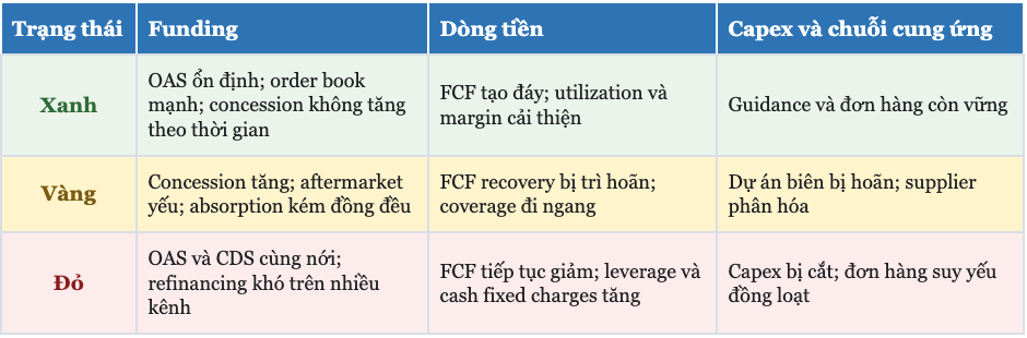
The warning only turns red when weakness appears simultaneously in cash flow, financing conditions, and real investment:
Projected FCF is lowered for multiple consecutive quarters.
OAS and CDS continue to widen after removing the effects of interest rates and general volatility.
Projects are delayed because the cost of capital or required rate of return increases.
Banks and private credit funds reduce limits or require more equity.
Hyperscalers cut capex, dragging down the orders and business prospects of suppliers.
Conversely, the risk thesis will weaken if FCF bottoms out, capacity utilization rises, and new bonds are absorbed without requiring increasingly large concessions. In that case, leverage can stabilize even if capex remains high.
Capital market conditions can be divided into three states:
Abundant: Most projects can access capital with low yield spreads.
Selective: Capital remains available, but is concentrated on strong companies and projects with clear cash flows.
Forced allocation: The cost of capital rises to the point where companies must cancel, sell, or delay projects.
→ A macroeconomic shock only begins in the third stage, when a repricing in financial markets forces companies to cut investment, reduce orders, and lower demand in the real economy.
Currently, the system has moved out of the abundant state and entered the selective phase. The distance to the forced allocation state remains significant, but this transition period will determine whether credit concerns remain confined to the bond market or develop into a broader investment shock.
CONCLUSION - THE TECHNOLOGY MAY BE RIGHT, BUT THE TIMING MAY STILL BE WRONG
The AI cycle is not like a traditional credit crisis. The core companies remain profitable, cash-rich, and highly rated. Demand for the technology is real, and the potential for lower computing costs opens a logical path for FCF recovery.
However, good technology does not automatically create a good financing structure. Capex is being deployed ahead of revenue, interest rate sensitivity has shifted to the bond market, and a portion of leverage is embedded in leases, purchase obligations, suppliers, and private credit.
The most easily misunderstood point is the scale of debt. Public bonds only show the most visible layer of capital. To fully assess it, three questions must be connected:
how much have hyperscalers committed to spending;
how much have suppliers borrowed based on those commitments;
what cash flow must materialize, and when, for the entire structure to be self-liquidating.
The market is not currently signaling a crisis. Bonds are still selling, leverage remains manageable, and consensus forecasts still expect FCF to rebound strongly from 2028. However, declining coverage ratios, widening yield spreads and CDS, and increasing long-term supply indicate that the era of nearly unconditional capital has ended.
→ The biggest risk is not that AI fails completely. It is that AI succeeds more slowly than the schedule that credit markets, long-term contracts, and infrastructure projects are relying on.
If FCF catches up to capex, the current repricing will merely be the normal cost of a major build-out cycle. If cash flows continue to be pushed back while leverage accumulates across multiple layers, the market will force companies to choose between projects rather than funding all their ambitions.
Ultimately, the limit of the AI race may not be the number of chips produced or the gigawatts of power connected to the grid. The limit may be the time that capital providers are willing to wait for those assets to prove their ability to generate cash.