Ample Reserve, QT and the Future of the Fed Balance Sheet

If you missed the best recent articles:

• Tesla: Billion-Dollar Gamble with Autonomous Vehicles and Robots

• Liquidity Crisis: Yes or No

• Nobel 2025: Republic of Knowledge - Republic of Knowledge 2.0

• US Banks Q3/2025: When Wall Street Accelerates Again

• Gold: Debasement Trade and the Era of Uncertainty

• What Factors Affect Mortgage Rates?

• Argentina and Dollarization

“Every banker knows that if he has to prove he is worthy of credit, however good may be his arguments, in fact his credit is gone.”
- Walter Bagehot, Lombard Street (1873)

(Excerpt from the most legendary bedside book in the history of modern central banking and finance thought)

Nearly 150 years later, that statement still holds true. Whenever the Fed has to prove that the system still has “ample” liquidity, liquidity has actually run dry.

There are systems that don't die from lack of money, but from money no longer flowing to the right places.

Since after 2008, we've been used to an America with “excess liquidity”: QE after QE, Fed balance sheet ballooning from under 1,000 billion USD to over 8,000 billion USD, banks flooded with reserves, money market funds parking trillions in ON RRP. Textbooks began talking about a “new regime” – the era of Ample Reserve – where the Fed can control interest rates just by a flick of the wrist in the IORB – ON RRP corridor without needing to pump – drain every morning like in the scarce reserve days before GFC.

But by October 2025, that model that seemed as solid as bedrock began to creak. ON RRP – the “buffer reservoir” that once held 2.5 trillion USD – nearly drained. SOFR started trading tight, then occasionally spiked above IORB – something that in theory floor system only happens when reserves have reached the efficient level. By month's end, liquidity hotspots reappeared: dealers couldn't turn money, MMFs had no buffer left, banks had to knock on the Fed's Standing Repo Facility door. That's no longer technical fluctuations. That's the signal: Ample Reserve system is hitting the ceiling.

The irony is that the Fed didn't hit the ceiling because of “sucking too hard” but because fiscal sucking up too much. When the Treasury has to issue debt to fund deficits over 7% GDP, each new T-bill issuance is like a vacuum suck into the banking system: money flows to TGA, reserves contract, repo strains. If RRP is still thick, pain isn't felt. But when RRP is down to 0, every USD drained hits reserves directly. At that point, the Fed no longer asks: “We want to shrink the balance sheet to what extent?” but must ask: “The system can withstand how much more without repeating 2019?”

That's why, the FOMC's October 2025 decision to stop QT is not a pivot, not “Fed U-turn”, and certainly not “starting new QE”. It's a maneuver to protect liquidity infrastructure. The Fed stopped not because they beat inflation, but because they saw exactly what Lorie Logan warned about: “Money market rates have risen to, and sometimes above, IORB - signaling that reserves have reached an efficient level.” In plain English: hit the floor already, withdraw more and the pipe bursts.

And this is the most important point of the week: when the Ample Reserve system had to stop QT just because repo started creaking, the question is no longer “Can the Fed continue shrinking the balance sheet?”, but “from now on, how will they manage the balance sheet to both support repo, support fiscal, and not be accused of QE?”. That's when the concept Quantitative Optimization (QO), terminal balance sheet, and deals that sound very harmless like Reserve Management Purchases takes the stage. The Fed won't print money en masse, but buy T-bills in drips, open the repo valve at the right time, gradually withdraw long-term MBS, rebuild a balance sheet less “political” but more “liquidity technical”.

This week, Viethustler will walk you through each part of the new era of the liquidity system:

• Why is a system called “ample” so... scarce?

• Why stop QT at $6.6 trillion is technical threshold, not policy threshold?

• Why is US fiscal policy 2025 pushing the Fed from “interest rate operator” to “artificial lung of the system repo”?

• And most importantly: the future of Fed balance sheet will no longer be cyclical expansion-deflation, but slow, purposeful expansion to sustain a debt market that can no longer stand on its own.

This article is not just about the Fed. It is about the new era of US liquidity – an era where the balance sheet is no longer a stimulus tool, but infrastructure to prevent the system from strangling itself.

1. The Ample Reserve System and why it is hitting limits before the October FOMC

1.1. The Shift in Operating Framework (Operating Framework)

Before the 2008 financial crisis, US monetary policy operated in a Scarce Reserve environment (Scarce Reserve Framework) – a mechanism where the Fed controlled interest rates by regulating the volume of reserves in the banking system.

At that time, the total reserves held by commercial banks at the Fed were just enough to meet required reserves (Required Reserves), with almost no excess. Therefore, a small change in reserve supply – just a few billion USD – was enough to cause the interbank interest rate (Federal Funds Rate) to fluctuate sharply.

In this model, the Fed did not set interest rates directly, but regulated them indirectly through open market operations (Open Market Operations – OMOs). Every morning, the Desk at the New York Fed would buy or sell a small amount of Treasury bonds to inject or drain reserves. When reserve supply increased, overnight rates fell; when supply decreased, rates immediately spiked.

This “quantity-based regulation” mechanism worked effectively when the Fed's balance sheet was small (under $900 billion USD), but it also made the system extremely sensitive to liquidity fluctuations. Just a deviation in Treasury cash forecasts or large interbank payment flows could push the interbank market into stress within hours.

*** It was precisely that fragility – along with the 2008 liquidity collapse – that forced the Fed to restructure its entire operating mechanism.

Post-crisis, Quantitative Easing (QE) programs worth trillions of USD caused bank reserves to balloon unprecedentedly. The market was no longer “short of money” but in a state of “chronic money surplus” (persistent liquidity glut). At that point, buying or selling a few billion USD in bonds was no longer enough to influence short-term rates, rendering the “quantity-based regulation” model ineffective.

The Fed was forced to switch to a “price-based regulation” mechanism (price-based regime) – known as the Ample Reserve Framework. In this new model, the Fed does not fix the reserve size but sets an interest rate corridor (interest rate corridor) to control short-term funding costs.

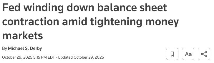
The core of this corridor is the “floor system” model – where money market rates (SOFR, repo, Fed Funds) are anchored tightly within a band defined by two key interest rate tools:

• IORB (Interest on Reserve Balances) – the rate the Fed pays on reserves banks hold at the Fed, acting as the upper floor.

• ON RRP (Overnight Reverse Repo Facility) – the rate the Fed pays to non-bank institutions, acting as the lower floor.

1.2. The Two Core Tools in the Model Floor System

(a) IORB – Interest on Reserve Balances

This is the rate the Fed pays on reserves that commercial banks hold at the Fed, officially applied from October 2008 – when the market was flooded with liquidity after the global financial crisis (GFC).

Previously, in the scarce reserve regime, market rates (Federal Funds Rate) fluctuated sharply due to small changes in reserve amounts. But after the Fed implemented large-scale asset purchase programs (Large-Scale Asset Purchases – LSAPs), bank reserves surged from less than $10 billion pre-crisis to over $800 billion in early 2009, and continued climbing through multiple QE rounds.
When money in the system became “chronically abundant”, quantity-based regulation (OMOs) lost effectiveness - even if the Fed injected or drained tens of billions of USD, rates didn't budge.

To restore control over short-term funding costs, Congress granted the Fed the authority to pay interest on reserves (Interest on Reserve Balances – IORB).
This mechanism establishes the upper floor in the interest rate corridor: if market rates (SOFR, Fed Funds) are lower than IORB, banks will choose to deposit at the Fed instead of lending externally - because it's absolutely safe and offers equivalent yield.

In other words, the Fed shifted from “lender of last resort” in times of scarce liquidity to “borrower of last resort” in times of abundant reserves.

(b) ON RRP – Overnight Reverse Repo Facility

Born in 2013, ON RRP is a tool that extends the Fed's “liquidity arm” beyond the banking sector, allowing Money Market Funds (MMFs), Government-Sponsored Enterprises (GSEs), and non-bank institutions to deposit overnight funds directly at the Fed.

In terms of mechanism, MMFs “lend to the Fed” overnight by temporarily purchasing Treasury securities from the Fed, and the next morning the Fed buys them back at a fixed yield – which is the ON RRP rate. This yield creates a sub-floor in the interest rate corridor: when market liquidity is flooded, non-bank institutions can deposit safely at the Fed instead of accepting lower rates in the private sector.

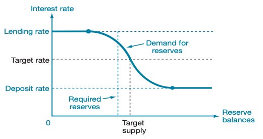
The chart below illustrates how ON RRP and IORB form two “anchor points” of the Floor System. Market rates (SOFR, EFFR) fluctuate within a narrow range sandwiched between these two levels, helping the Fed control short-term funding costs even as the balance sheet expands by trillions of USD.

Thanks to the two-floor mechanism – IORB (upper floor) and ON RRP (lower floor) – the Fed maintains complete control over market interest rates without needing to pump-suck liquidity daily as in the era of reserve scarcity.

1.3. “Ample” Does Not Mean “Infinite”: Experimental Limits & 2019 Lessons

After more than a decade of experimentation, the Fed drew a costly conclusion: “ample” is not “abundant.”
A healthy liquidity system does not need infinite reserves, but an efficient equilibrium level - enough to absorb shocks, but not so excess as to paralyze market functions.

Story: Repo Shock 2019

• Context: QT 2017–2019 reduced the Fed's balance sheet by nearly $700B, system reserves from peak ~$2.8T$ down to ~$1.38T$.

  

• Trigger: At the same time, the Treasury increased bond issuance, drawing more money into the Treasury General Account (TGA) – causing bank reserves to drop suddenly.

• Consequence: Within 48 hours, the overnight repo market faced severe liquidity shortage. Repo rates spiked from ~2% to 10%, far exceeding the Fed's target rate.

  

• Response: The Fed was forced to intervene urgently - injecting over $75B via repo operations each day and then restarting T-bill purchases on a $60B/month scale (a form of “short-term QE”) to restore liquidity.

  

Ample but Efficient – the new philosophy of the balance sheet.

Dallas Fed President Lorie Logan states that the Fed's goal is not to shrink or expand the balance sheet, but to optimize it (Quantitative Optimization).

• If reserves too low → repo rates exceed IORB → liquidity stress.

• If reserves too high → repo falls below IORB → system stagnates, capital does not leave the Fed.

➡️ The ideal balance is when TGCR, SOFR fluctuate around IORB - reflecting stable and safe “liquidity blood pressure”.

The chart below – from BofA Global Research – illustrates the reserve demand curve in the Fed's ample reserve regime.

Horizontal axis is bank reserve levels (reserve balances), vertical axis is money market rates.

• In the Abundant region, reserves too plentiful cause TGCR to lie below IORB - excess liquidity, rates stuck at the floor.

• As reserves gradually drain to Ample, TGCR approaches IORB – indicating the market is at the “efficient equilibrium point”.

• If continuing to drain liquidity into the Scarce region, TGCR jumps above IORB - sign of market money shortage, repo stress appears.

The red dot “Logan ideal” represents exactly the state described by Lorie Logan in her speech:

“Money market rates have risen to, and sometimes above, IORB - signaling that reserves have reached an efficient level.”

“Money market rates have risen to, and sometimes exceeded, IORB levels - signaling that system reserves have reached an efficient threshold.”

In other words, this chart is the Fed's “liquidity map” – where just one overstep causes the system to slide from balance to stress.

That's also why the FOMC in October 2025 decided to end QT: The Fed does not want to repeat the 2019 repo stress trajectory, when the system crossed the “ample” boundary unnoticed.

1.4 Real-World Manifestations of Reserve Stress at the October FOMC

In October 2025, Dallas Fed President Lorie Logan affirmed in her speech “Ample Liquidity for a Safe and Efficient Banking System” that the Fed has approached the technical balance level.

“Money market rates have risen to, and sometimes above, IORB - signaling that reserves have reached an efficient level. It is the right moment to end asset runoff.”

“Money market rates have risen to equal, and even exceeded, IORB - indicating that reserves have reached the efficient threshold. This is the right moment to end the balance sheet reduction process (asset runoff).”

She said bluntly: the system has reached the final “ample” threshold – where every subsequent liquidity withdrawal could push the market into “scarce” status. The Fed no longer has room to continue QT without risking loss of control over short-term interest rates.

Logan describes the operating framework as a liquidity triangle between the Fed – the banking system – and the US Treasury:

• When the Fed implements QT, reserves are withdrawn from the system.

• When the Treasury issues new debt, money flows are further sucked into Treasury General Account (TGA).

• During the 2022–2024 period, excess funds at Reverse Repo Facility (RRP) served as the buffer absorbing those shocks.

• But by the end of 2025, this buffer is nearly empty, causing every capital drain to hit directly at commercial banks' reserves.

(1) ON RRP – the last buffer – depleted.

ON RRP, which once peaked above 2.5 trillion USD, now only a few tens of billions - a record low.

This means: the “non-bank buffer” has disappeared. From now on, every capital withdrawal – whether from QT or Treasury bond issuance – hits directly at commercial banks' reserves.

The chart below clearly illustrates this process: the green part is Reverse Repo Facility (RRP) expanding during 2021–2023 then plunging straight down near 0, while the red part – Standing Repo Facility (SRF) – starts to sprout up again.

Notably, the enlarged frame in the bottom corner shows the largest spike since the pandemic, not at quarter-end – meaning the market has to use the Fed's “lifeline” even in normal conditions.

(2) SOFR exceeds IORB ceiling.

The standard repo rate (SOFR) frequently trades at or above IORB, reflecting intense competition to hold short-term capital.
This is the classic signal of a system stepping out of the “ample” zone into “tight liquidity” – where borrowers must pay extra fees to attract the remaining money flows in the system.

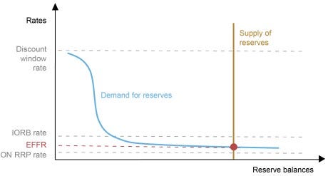
(3) Liquidity hotspots reappear (repo chart):

At month-end and quarter-end points, the repo volume that banks must borrow directly from New York Fed via Standing Repo Facility (SRF) surges, with some sessions exceeding $10 billion USD.

This is clear evidence that the internal market cannot circulate money – must resort to the Fed's “lifeline”. This scene recalls the shadow of 2019, only this time, system-wide reserves are significantly lower.

This chart not only shows the market is thirsty for money; it shows the system is breathing on a “liquidity support machine” – and that machine is the Fed.

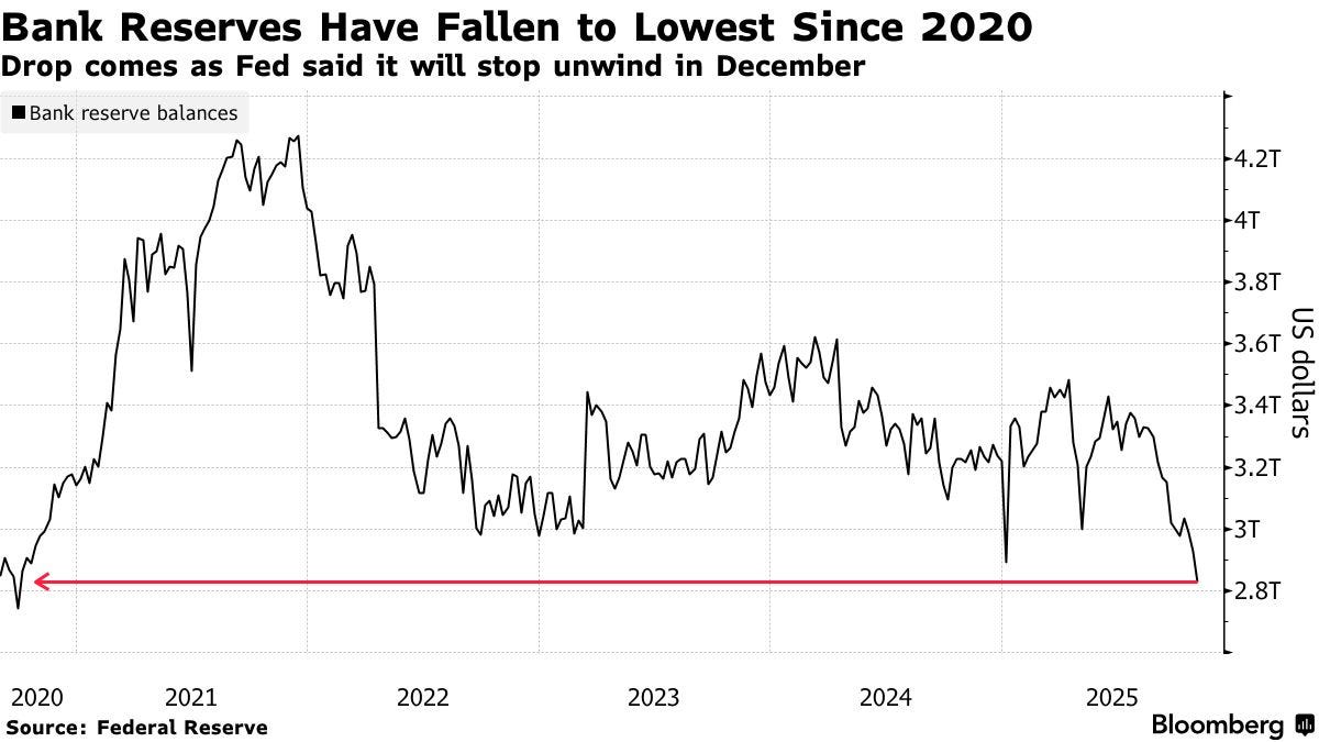
Additionally, total bank reserves at the Fed are now around $2.8–3.0 trillion USD, sharply down from the post-pandemic peak of $4.3 trillion USD – a zone where every additional USD withdrawn can trigger chain reactions in the repo market.

In other words, QT has reached the very edge of the “ample” zone. One more step, and the system will slide into “scarce” state, where even a single money shift between banks, MMFs, and Treasury General Account (TGA) can amplify into an interest rate spike. At this threshold, stopping QT is not easing, but preempting a repo shock that the market has already begun to price into the data.

Keeping the system in “ample but not excessive” state allows the Fed to regulate capital costs through the interest rate corridor (IORB – ceiling, ON RRP – floor, SRF – lifeline) without needing “emergency money pumping” like in 2019. That is the truly sustainable state of the Ample Reserve Framework – where the Fed regulates not by size, but by the structure and rhythm of liquidity circulation.

→ Right at that fragile balance threshold, the October 2025 FOMC had to act. The Fed did not stop QT to ease, but because the “liquidity pipeline” has started screaming - a signal that the system is silently thirsty. If not stopped, the market will force them to stop – and then, the cost will not just be a repo shock, but a crisis of confidence in the US monetary mechanism.

2. October FOMC Decision: Stopping QT and the Rift Within the Leadership

The October 2025 FOMC meeting was a double turning point - an event characterized by dichotomy, where two technically easing actions come with a clear tightening message.

The Fed both cut rates by another 25 basis points (bringing the range down to 3.75–4.00%), and officially announced stopping QT, but Jerome Powell's words stunned the market: he spoke like a “hawk” right at the moment of acting like a “dove”.

2.1. Technical Decision: Stopping Quantitative Tightening (QT)

A “technical pivot” step, not a “policy pivot”

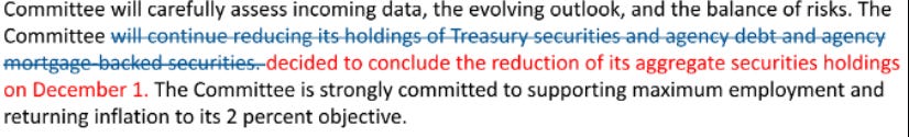
The decision to stop the Quantitative Tightening (QT) program from 1/12/2025 is a technical turning point with systemic consequences. Fed did not announce this as an easing policy, but as a liquidity risk-management action.

After nearly three years of net withdrawal of liquidity from the system, Fed has reached the lowest possible threshold without breaking the “Ample Reserve” framework – in other words, has approached LCLoR (Lowest Comfortable Level of Reserves).

In the press conference, Powell acknowledged “monetary and financial conditions have tightened significantly in the past three weeks”, a subtle but clear hint that SOFR and repo rates are showing stress signs similar to the pre-crisis 2019 period.
Fed understands that continuing QT would cause bank reserves to fall below the safe zone, triggering short-term interest rate loss-of-control risk - something they cannot allow to happen a second time.

Systemic risk management: protecting the monetary operating framework

The move to stop QT is therefore seen by experts as a “preemptive repo shock action”, a measure to protect liquidity infrastructure rather than changing monetary policy direction.
Fed accepts keeping the large balance sheet at ~$6.6 trillion USD - equivalent to 22% US GDP - as the price to maintain stability of the “ample reserve” operating framework.

This means Fed has closed the QT 2022–2025 book, but has not yet reopened QE.
The market calls this “technical pause”, but in the language of market makers (dealers), it is a breath out – “exhale moment” – of the suffocating liquidity system.

“Terminal Balance Sheet”: Completing the post-pandemic deleveraging phase

Stopping QT at the $6.6T scale is seen as a sign that Fed has reached the balanced reserve threshold between:

• commercial banks' operating reserve demand,

• TGA size fluctuating 500–700 billion,

• and “ample” reserve levels to maintain repo market stability.

From here, Fed's Balance Sheet enters the “structural normalization” phase (portfolio normalization): instead of further shrinking, Fed will restructure holdings, gradually reducing MBS and increasing T-bills proportion to regain flexibility.

In summary, QT ends not because Fed wants to ease, but because they have reached the technical limit of the system they designed themselves.

2.2. Divisions and Hawkish Message

If the decision to stop QT is a technical action, then Powell's message is a political – monetary declaration:

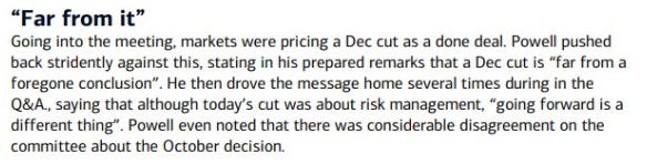
“Further cuts in December are not a given – but a very remote assumption.”

This statement, seemingly an ordinary warning, caused the market to reprice the entire yield curve in just a few hours.

“Dual signal”: Cutting rates – but raising real rate expectations

• Fed cuts nominal rates 25bps, but the “no commitment to further cuts” message causes long-term yields to rise sharply, pushing real yields (real yield) to the highest since 2022.

• This is a typical policy paradox: Fed acts dovish but speaks hawkish – a deliberate tactic to avoid loosening financial expectations too early.

Powell seems to be trying to anchor inflation expectations while maintaining Fed's credibility amid increasing political pressure from the White House and Treasury on “stabilizing borrowing costs”.

Internal rift – first time since 2018

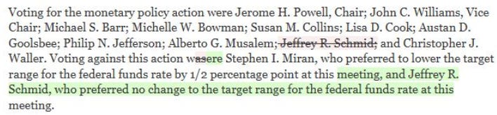
For the first time in six years, the FOMC decision did not achieve unanimous consensus.

• The “dove” wing (Miran) wanted deeper cuts (50bps) to respond to weakening growth and credit signals.

• The “hawk” wing (including Logan, Schmid, Hammack) opposed, arguing that core inflation remains persistent and the labor market remains tight.

The existence of “two-sided dissents” - with members wanting more easing and others wanting to hold - reflects a Council divided along data lines.

In other words, Powell no longer has full control over internal expectations direction, and Fed has entered a “data-dependent but directionless” policy phase - which makes markets more volatile than ever.

3. Future of Balance Sheet: QT Framework Closed, Restructuring Game Begins

When Fed ends QT on 1/12/2025, they are not only stopping a liquidity withdrawal cycle, but actually putting an end to the “shrinking at any cost” era.

From that point, monetary policy moves to chapter three of the modern balance sheet cycle – the structural optimization phase instead of size reduction.

If the 2022–2025 phase was “forced weight loss”, then the upcoming phase is “muscle reallocation” – an accurate metaphor for what Fed plans to do with its $6.6 trillion portfolio.

3.1. Fixed Size (Terminal Size)

Stopping QT at $6.6 trillion USD marks an implicit statement that Fed has reached the technical equilibrium point of the Ample Reserve Framework - where liquidity is sufficient to keep the system safe, but no longer excess to push rates below the policy corridor.

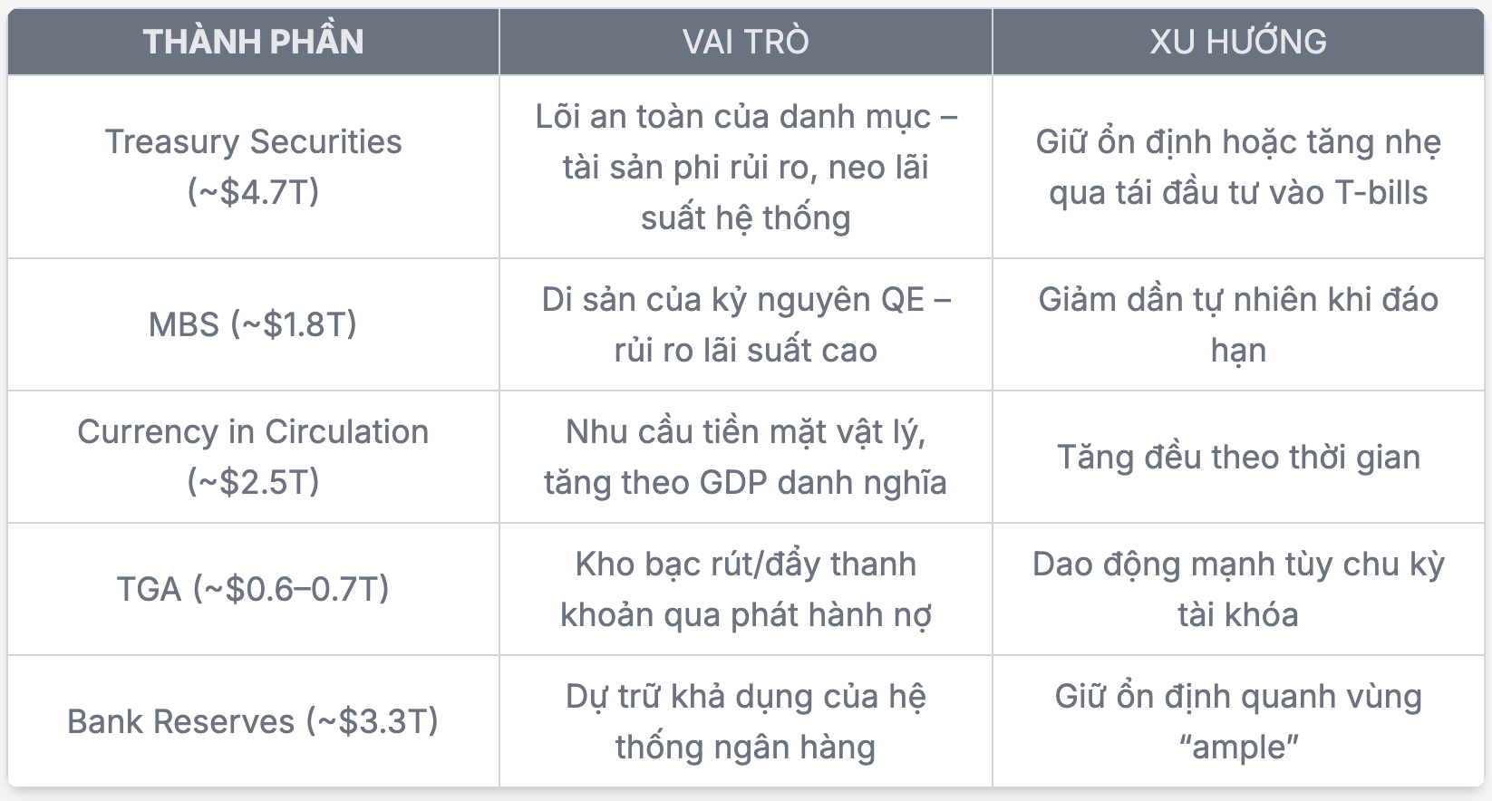
The chart below clearly shows that balanced structure on Fed's balance sheet:

🟡 Bank Reserves (~$3.0–3.2 trillion USD)

This is the blood of the financial system. Bank reserves have dropped sharply from the post-pandemic peak of $4.3 trillion to near the bottom of the ample. At this level, the system still operates stably, but just a capital withdrawal from the Treasury or MMFs could push the market into a state of scarce, where short-term interest rates lose control.

🟣 TGA (~$0.6 trillion USD) maintains in the “fiscal stability” zone

The Treasury account is the “control valve” between fiscal and monetary. When TGA increases, it sucks money out of the system; when it decreases, it returns reserves to banks. The $0.6–0.7 trillion level allows the Treasury to maintain operations without strangling liquidity, but each large bond issuance can still cause short-term waves in the money market.

🔴 RRP (~$0.1–0.3 trillion USD) nearly depleted

Reverse Repo Facility was once a giant non-bank liquidity “reservoir” with over $2.5 trillion in 2022, now nearly empty. When MMFs withdraw from RRP to buy T-bills and lend back in repo, this buffer disappears – every liquidity withdrawal now directly impacts bank reserves.

🟢 Currency in Circulation (~$2.5 trillion USD)

Currency in circulation is an inelastic factor, increasing steadily with nominal GDP. Each year, this amount gradually drains reserves from the system – a natural, slow but continuous process, forcing the Fed to replenish with technical liquidity if it doesn't want the “money pipeline” to dry up over time.

To understand better equilibrium structure this, we can look at the detailed components of the balance sheet at “Terminal Size”:

From this picture, it can be seen: Terminal Size is not a static number, but a dynamic equilibrium state between three major forces:

1. QT – the process of gradually withdrawing reserves from the system;
2. Treasury debt issuance (Treasury issuance) – sucking liquidity back through the fiscal channel;
3. Natural reserve demand – reflecting the defensive balance sheet behavior of commercial banks.

At the current scale, reserves account for about 12% of nominal GDP, just enough to prevent a 2019-style repo shock, but not enough to absorb another large capital withdrawal.
The Fed is in the “ample but not excessive” zone – where every billion USD withdrawn can amplify into large fluctuations in short-term funding costs.

Thus, Terminal Size is not a static number - but a dynamic equilibrium state between three forces: QT (liquidity withdrawal), debt issuance (Treasury issuance), and natural reserve demand.

“Dynamic equilibrium” – the central concept of post-QT

The Fed cannot fix an absolute reserve level; what they manage is the safe fluctuation range (comfort band).

Any shock – TGA increase, RRP fluctuations, or shifts between MMFs and banks – can push the system out of the “ample” zone.

The Fed's task from now on is to finely coordinate cash flows between the pipelines, not to expand or contract the balance sheet further.

3.2. Portfolio Recomposition (Portfolio Recomposition): From QE to “QO” (Quantitative Optimization)

When the Fed announces stopping QT, the next question is no longer “when to restart QE”, but “how will the Fed restructure the balance sheet to preserve liquidity flexibility?”.

Instead of expanding the size, the Fed enters a new phase – Quantitative Optimization (QO) – where the focus is on the quality and structure of the balance sheet, not the absolute size.

(a) Prioritizing T-Bills: Returning to “liquid, short, and neutral” assets

In the post-QT phase, the Fed is gradually redirecting reinvestments of maturing and prepayment MBS to short-term Treasury bills (T-bills) – a strategic turning point rarely mentioned but with enormous mechanical implications for liquidity structure.

There are 3 very clear reasons:

First, T-bills are an asset type of “liquid, short, and neutral”: highest liquidity among government debt instruments, almost no duration risk, and sends little policy signals. When the Fed buys T-bills, the market does not see it as “QE for easing”, but only as technical adjustment to stabilize reserves. Unlike holding long-term bonds (Long-term Treasuries) or MBS, T-bills allow the Fed to expand the balance sheet without distorting the yield curve – a very sensitive factor in the current context.

Second, the current portfolio structure is seriously imbalanced. In the total portfolio of about $4.2 trillion USD in Treasury bonds, T-bills currently account for only ~$200 billion – equivalent to less than 5%, much lower than the “normal” level before QE. Meanwhile, long-term bonds (over 10 years) account for nearly 38% – a record high, reflecting the “prolonged legacy” of QE periods when the Fed deliberately concentrated on buying long-term debt to lower yields. As a result, the Fed's balance sheet today has high duration and low flexibility – a paradox when they need quick response capabilities in a volatile liquidity environment.

Third, the Fed needs to “shorten duration” to regain maneuverability. Gradually increasing T-bill holdings will help the Fed restructure the balance sheet into a true “liquidity buffer” – that is, a technical buffer that can expand or contract flexibly according to the reserve needs of the banking system. When liquidity stress appears, the Fed can quickly reinject through repo or sell T-bills without creating long-term yield shocks.

→ This is how the Fed turns the balance sheet into a “liquidity buffer” instead of a “policy lever” – a self-regulating buffer instead of a stimulus tool.

(b) Reduce MBS: Escape from the QE legacy

Alongside increasing the T-bill weight, the Fed will let the mortgage-backed securities (MBS) portfolio mature naturally without reinvestment – gradually moving towards the “All-Treasury Portfolio” goal, i.e., a portfolio entirely consisting of Treasury bonds.

First, this is the process of “deconstructing the QE legacy”.

Throughout the 2009–2021 period, the Fed became implicit sponsor for the US real estate market, by buying more than $2.7 trillion USD MBS to lower mortgage rates and stimulate consumption. That had political and economic reasons – saving the credit system after the housing crisis – but today it has left a huge “duration risk legacy”:

• The average duration of the MBS portfolio is much longer than Treasuries, making the Fed's balance sheet sensitive to yield fluctuations.

• Prepayment cash flows (when borrowers pay off early) make the reserves the Fed receives unpredictable – a major technical risk in liquidity management.

• And most importantly, the Fed is pushed into a political role: indirectly influencing house prices, contrary to the “asset neutrality” principle.

Second, exiting MBS is a step to separate the Fed from housing industrial policy.

When the Fed stops reinvesting, the amount of MBS in the portfolio will naturally decrease according to the repayment rate, helping to reduce exposure to the most politically sensitive sector of the economy. This restores the neutrality of the balance sheet – where the Fed's assets only reflect government debt obligations, not the risk structure of American households.

Third, lessons from the 2020–2023 period.

During the post-pandemic QE period, the Fed both injected reserves and inadvertently created a burden of interest on reserves costs up to hundreds of billions of USD per year. The lack of clear boundaries between QE for stimulus (monetary stimulus) and QE for market stabilization (market functioning) led to policy misinterpretation – and the balance sheet ballooned far beyond liquidity targets.

Therefore, the MBS reduction strategy is not just a technical move, but a policy statement:

The Fed is withdrawing from the role of “pricing household credit risk”, to return to its neutral essence – a central bank that only holds government debt, manages liquidity, and stabilizes short-term interest rates.

→ This is a necessary step for the Fed to escape the “long shadow of QE”: shifting from a stimulus-oriented balance sheet to a stability-oriented one, where every reserve flow is due to market demand – not political targets.

(c) “The Long Game”: Natural expansion, not QE

In the long term, the Fed's balance sheet will continue to expand “naturally” (organic growth) - not for economic stimulus like previous QE periods, but simply because the US economy and global liquidity demand are growing larger.

The concept of “Reserve Management Growth” that the Fed emphasizes from 2025 onward describes it accurately: the balance sheet will increase gradually by about 5% per year, equivalent to the nominal growth rate of the US economy, to ensure that reserves in the system grow with GDP scale.

• Orange line (Nominal GDP) represents the nominal growth of the economy,

• Blue line (Fed Balance Sheet) represents the balance sheet size.
  Projections show that after the 2022–2025 contraction phase, the balance sheet will stabilize around $6.5–7 trillion USD, then increase again at a rate of ~5%/year – a “natural growth path” instead of the expansion shocks like previous QE periods.

First, three main drivers explain this trend:

• Currency in Circulation continues to increase along with nominal GDP, reflecting the real economy's demand for holding cash and physical payments. Each USD in circulation in society corresponds to a liability on the Fed's balance sheet - and therefore, the balance sheet must be larger to “accommodate” that portion.

• Expanding banking system: increasing scale of assets, payments, and market cap leads to higher demand for safe reserves to meet liquidity requirements, comply with Basel III, and address market risks.

• Technical factors like Treasury General Account (TGA) and RRP remain at levels higher than pre-GFC, making the overall balance sheet size unable to return to “pre-crisis” levels but instead stabilize at a new high baseline.

Second, the end of QT is not a stopping point - but a stabilization point. Data from Fed and BofA shows: after QT stops at the end of 2025, the size of the SOMA (System Open Market Account) portfolio - i.e., the amount of bonds held by the Fed - will stabilize around $6.5–7.0 trillion USD, before gradually increasing again at the pace of US economic growth.

• In the “higher reserve share” scenario (green line), the Fed holds more reserves relative to nominal GDP - reflecting a cautious liquidity environment.

• In the “lower reserve share” scenario (blue line), the Fed allows reserves to decrease slightly, but the balance sheet still grows with the economy's scale.

Both scenarios yield a common result: no more balance sheet contraction like the 2018–2019 period, but stabilization and expansion according to the natural cycle.

Third, the shift to the “era of the permanent balance sheet.” The Fed's securities holdings ratio to nominal GDP (NGDP) is expected to remain around 20–25% -
lower than the pandemic peak (~40%), but still double that of the pre-GFC era (~10–12%).
This means: large size is no longer a sign of easing (QE), but the operational baseline of the US financial system.

“The Fed will have to increase its Treasury holdings over time, so that the supply of reserves keeps pace with economic growth.”

- Former Fed Vice Chairman, Bill Dudley

In summary, the Fed no longer “inflates to rescue” like in the QE era, but “grows to operate” (Quantitative Optimization – QO).

→ This is a transformation from active policy (stimulative policy) to a self-balancing system (self-stabilizing system) - where the Fed's balance sheet becomes the technical backbone of global liquidity, no longer a temporary tool to cope with crises.

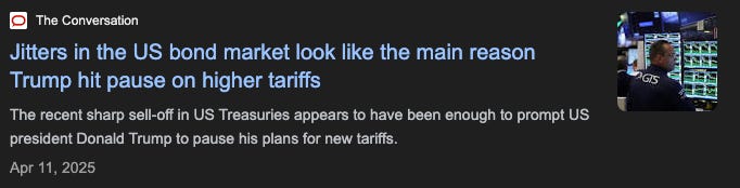
4. Impact on Treasury Bonds (UST): Technical Support for the Treasury & Defense Mechanism Against “De-Dollarization”

When the Fed ends QT, the US Treasury bond market (UST) is the first beneficiary - not because the Fed is “pumping money” back, but because a massive debt supply has been silently eliminated.

In the context of Washington struggling with a fiscal deficit of 2.3 trillion USD/year and record net issuance demand, stopping QT is a technical lifesaver for the Treasury, helping “prevent the system from strangling itself.”

4.1. Reducing Supply-Demand Pressure: Fed Withdraws, Treasury Breathes Easier

QT – when the Fed is the “silent seller”

Throughout the 2022–2025 period, the Fed has withdrawn more than $2.4 trillion from the balance sheet, equivalent to indirectly selling tens of billions of USD in Treasury bonds each month.
This forces the market to absorb a massive net supply simultaneously with the Treasury - two flows in the same direction, draining liquidity from the private sector.

When the Fed stops QT, that net selling flow disappears immediately. The bond market receives a “supply relief shock” - even if the Fed doesn't buy more, their stopping selling is enough to reduce the monthly absorption pressure by ~95 billion USD.

Liquidity support & control of “Term Premium”

By stopping liquidity withdrawal, the Fed slows the rise in long-term yields. This helps contain term premium - the risk premium that investors demand to hold long-term bonds – which has surged to its highest level since 2013.

In other words, the Fed is indirectly “insuring refinancing risk” for the US Treasury: keeping borrowing costs from sliding to unsustainable levels amid increasingly weak fiscal conditions.

“Liquidity multiplier”: When cash flow changes direction

• Previously, QT → reduced reserves → reduced demand for UST → increased yield.

• Now, stopping QT → stable reserves → keeps bank cash flow in the system → increases capacity to absorb new UST.

• → The Fed has invisibly shifted the system from “seller-driven” to “absorber-driven”, helping the Treasury market regain the necessary depth (depth).

4.2. “Public Debt Is Monetary Policy”: The New Fiscal-Monetary Linkage

Stopping QT cannot be read only through a monetary lens; it is an implicit fiscal decision. In a system where public debt has exceeded $38 trillion, the Fed is no longer an independent liquidity controller, but a compelled partner in the national financial balance chain.

Deficits and fiscal “Fed Put”

The Treasury needs to issue trillions of USD in new bonds to fund spending and refinance maturing debt.

If the Fed continues QT, demand will contract just as supply surges - a perfect recipe for a “yield crisis” (yield blowout).

Stopping QT thus becomes the Treasury's “Fed Put” – an implicit commitment that the Fed will not let government borrowing costs rise too quickly.

Even if the Fed doesn't buy debt directly, stopping sales is a deliberate form of technical support. The market understands this as “Shadow QE” – not injecting new liquidity, but removing a major liquidity drain. In other words, balance sheet policy has become a tool for fiscal stabilization.

When fiscal controls the balance sheet

The Fed can still set interest rates itself, but is increasingly losing control of the balance sheet to the budget deficit.

The Fed can still set interest rates as it wishes, but is gradually losing control of balance sheet policy to the ever-expanding budget deficit… Keeping repo rates stable will require the Fed to continuously expand its balance sheet, and in reality, handing back the decision on its size to fiscal authorities.

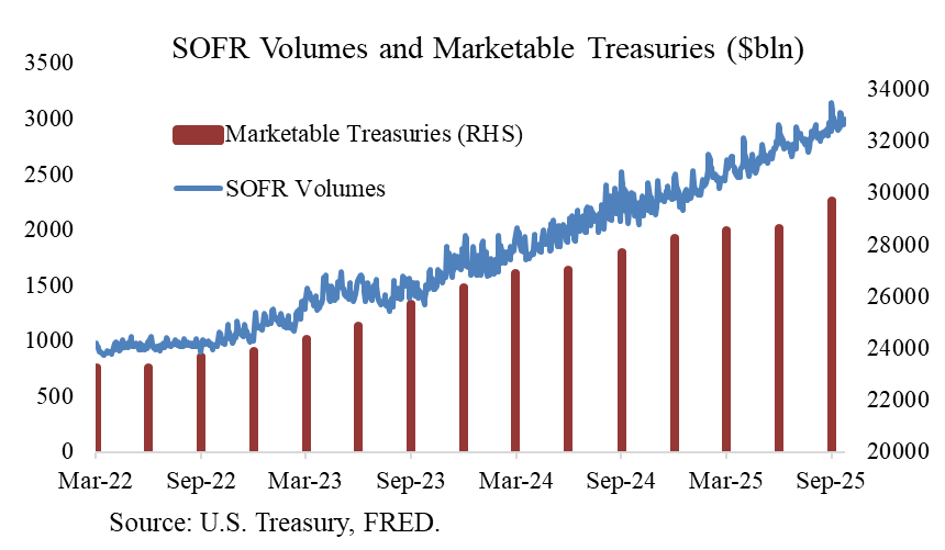
This is precisely the Balance Sheet Dominance phenomenon – when monetary policy is “taken hostage” by fiscal. Short-term borrowing demand (repo financing) is growing faster than the system's supply capacity, due to the $2 trillion annual deficit being largely funded by leveraged investors, especially basis trade funds – they buy Treasury bonds with repo borrowing. As the amount of outstanding bonds surges, repo demand becomes endless.

The chart below shows this clearly:

as the total tradable Treasury bonds (red) surge quarter by quarter, SOFR-standard repo trading volume (blue) also climbs in parallel. Repo market is expanding along with the deficit – and this is the “transmission channel” by which fiscal controls monetary liquidity.

At that point, to keep repo rate from spiking above IORB and breaking the interest rate corridor, the Fed is forced to expand its balance sheet periodically. In other words, the fiscal deficit is now forcing the Fed to inject more reserves – not because the economy needs it, but because the repo system needs it. That's when the Fed's balance sheet is no longer decided by the Fed, but shaped by the Treasury's financing needs.

Yields and political power

The 10-year UST yield has become America's “political window.” Every time it exceeds 5%, not only the market but also the White House, Treasury, and Fed come under pressure.

Powell understands that to maintain “nominal fiscal stability,” the Fed must cap the yield rise through technical actions: stopping QT to avoid publicly declaring QE.

The Fed no longer controls the money supply – they are controlling the credibility of Treasury bonds. And in a closed loop, public debt has now become monetary policy.

The Fed no longer operates the system on inflation targets, but according to the government's fiscal tolerance.
QT ends not because inflation has stabilized, but because the national balance sheet can't withstand another reserve withdrawal.

4.3. Geopolitical Perspective: Fed – The “Last Shield” Against De-Dollarization

As central banks in the BRICS bloc, ASEAN+, and Middle East gradually reduce the USD share in their FX reserves, maintaining UST yield stability becomes a geopolitical priority.

Global reserve trust competition

UST is not just a debt instrument – it is the foundation of the global USD.
If yields fluctuate sharply or lose liquidity, countries holding trillions of USD in reserves (China, Japan, Saudi Arabia) will accelerate diversification.
Stopping QT helps the Fed ensure that UST remains the “lowest risk asset in the financial universe,” anchoring the global monetary system.

“Monetary defense by liquidity design”

Instead of launching a new QE program (easily labeled “money printing”), the Fed chooses a more sophisticated defensive strategy: maintaining UST liquidity elasticity through stopping QT and portfolio restructuring.
By keeping the system “ample but elastic,” the Fed is protecting the USD through technical stability, not political statements.

Symbolic impact

In the world's eyes, this decision sends the message:

“The Fed will not let the UST market – the foundation of the dollar order – lose liquidity.”
This is not just a monetary declaration, but a commitment to protect the USD's power structure.

5. Conclusion

After three years of continuous withdrawals, QT policy has brought the US banking system to the technical edge of the Ample Reserve Framework model. Liquidity indicators – from SOFR hitting the IORB ceiling, periodic SRF drawdowns, to recurring repo stress at month-end and quarter-end – all sound a common signal: the “liquidity pipeline” is drying up. Just one more reserve withdrawal, and the system will slide into scarce territory, where short-term rates no longer follow the technical corridor but fluctuate randomly with each withdrawal from Treasury (TGA) or Money Market Funds (MMFs).

In that fragile state, the Fed stopping QT is not an easing action, but a move to protect the structure of the very system they designed. The Fed understands that every dollar of reserves is not just a balance sheet number, but red blood cells of the financial system. When that layer is too thin, just one TGA spike – the Treasury's sudden capital drain – is enough to make the repo market spasm for hours. That is the physical limit of the “ample” state – where even one drop of liquidity withdrawn can break the circulation of the entire financial body.

The next issue lies no longer with the Fed, but with fiscal.
When the Fed stops draining, the Treasury accelerates bond issuance to cover the >7% GDP deficit – that massive debt flow floods the repo market like a collateral tsunami.
Financial institutions are forced to borrow short-term to hold the pile of new bonds, driving reserve demand skyrocketing. The liquidity thirst is no longer technical, but a direct consequence of the fiscal structure. If the Fed doesn't replenish reserves, they risk losing control of short-term funding costs – as in the September 2019 lesson, when repo rates spiked fivefold in hours.

From my own forecast view, the Fed will almost certainly expand its balance sheet again in Q1/2026 – earliest January, latest March – via Reserve Management Purchases. They may net purchase ~35–50 billion USD bonds per month, equivalent to net expansion of 20–30 billion USD/month, while letting MBS mature naturally.

These trades will stabilize the repo market, reassure investors on public debt financing, and indirectly lower government borrowing costs. This isn't classic QE for growth stimulus, but mechanical QE – a “liquidity IV drip” to sustain breathing for the system choking under public debt weight.

Fed not easing – Fed just transfusing.

To meet growing reserve demand, they'll return to “periodic liquidity pumping,” but under technical cover. Three main tools on the table:

1. Buying T-bills – directly injecting reserves into banks, which then flow to repo, flexible and less “QE-flavored”;

2. Standing Repo Facility – safety valve for Fed short-term lending when market thirsty, though current scale small;

3. Natural balance sheet expansion, allowing reserves to grow with public debt to avoid 2019 repeat.

All lead to one conclusion: QT over, but Fed balance sheet must keep expanding – not politics, but liquidity physics.

When reserve demand stems from budget deficit, monetary-fiscal boundary dissolves. Fed no longer buys bonds for inflation control, but to keep system breathing. QT ends – not Fed wanting ease, but Washington leaving repo market breathless.

This time, liquidity machine starts not from crisis, but financial body accustomed to IV drip – artificial life sustained not by market's natural pulse, but central bank's technical hand.

P/s: TRUMP DEFINITELY WILL NOT PICK WALLER AS FED CHAIRRRR@@@